Shrinkage Estimators and Hierarchical Bayes

STA 721: Lecture 11

Merlise Clyde (clyde@duke.edu)

Duke University

Outline

• Lasso
• Bayesian Lasso

• Readings (see reading link)

  • Seber & Lee Chapter Chapter 12
  • Tibshirani (JRSS B 1996)
  • Park & Casella (JASA 2008)
  • Hans (Biometrika 2010)
  • Carvalho, Polson & Scott (Biometrika 2010)

LASSO Estimator

Tibshirani (JRSS B 1996) proposed estimating coefficients through \(L_1\) constrained least squares via the Least Absolute Shrinkage and Selection Operator or lasso \[\hat{\boldsymbol{\beta}}_{L} = \mathop{\mathrm{argmin}}_{\boldsymbol{\beta}} \left\{ \|\mathbf{Y}_c - \mathbf{X}_s \boldsymbol{\beta}\|^2 + \lambda \|\boldsymbol{\beta}\|_1 \right\}\]

• \(\mathbf{Y}_c\) is the centered \(\mathbf{Y}\), \(\mathbf{Y}_c = \mathbf{Y}- \bar{\mathbf{Y}} \mathbf{1}\)

• \(\mathbf{X}_s\) is the centered and standardized \(\mathbf{X}\) matrix so that the diagonal elements of \(\mathbf{X}_s^T\mathbf{X}_s = c\).

• use the scale function but standardization usually handled within packages

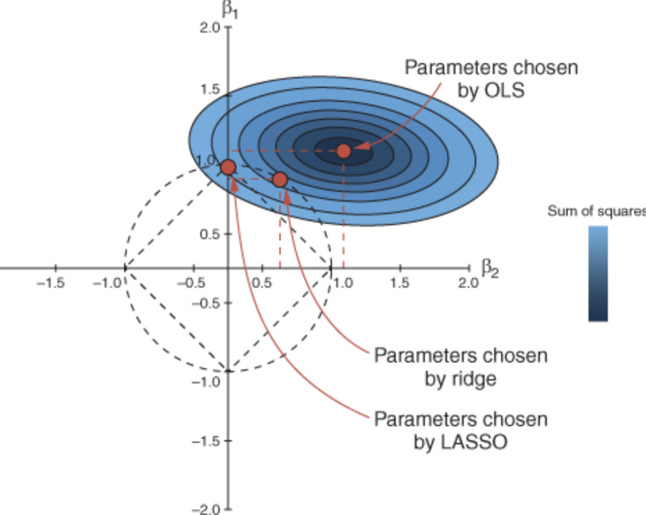
• Control how large coefficients may grow \[\arg \min_{\boldsymbol{\beta}} (\mathbf{Y}_c - \mathbf{X}_s \boldsymbol{\beta})^T (\mathbf{Y}_c - \mathbf{X}_s\boldsymbol{\beta})\]

  \[ \text{ subject to } \sum |\beta_j| \le t\]

Lasso Solutions

The entire path of solutions can be easily found using the ``Least Angle Regression’’ Algorithm of Efron et al (Annals of Statistics 2004)

library(lars); datasets::longley
longley.lars = lars(as.matrix(longley[,-7]), longley[,7], type="lasso")

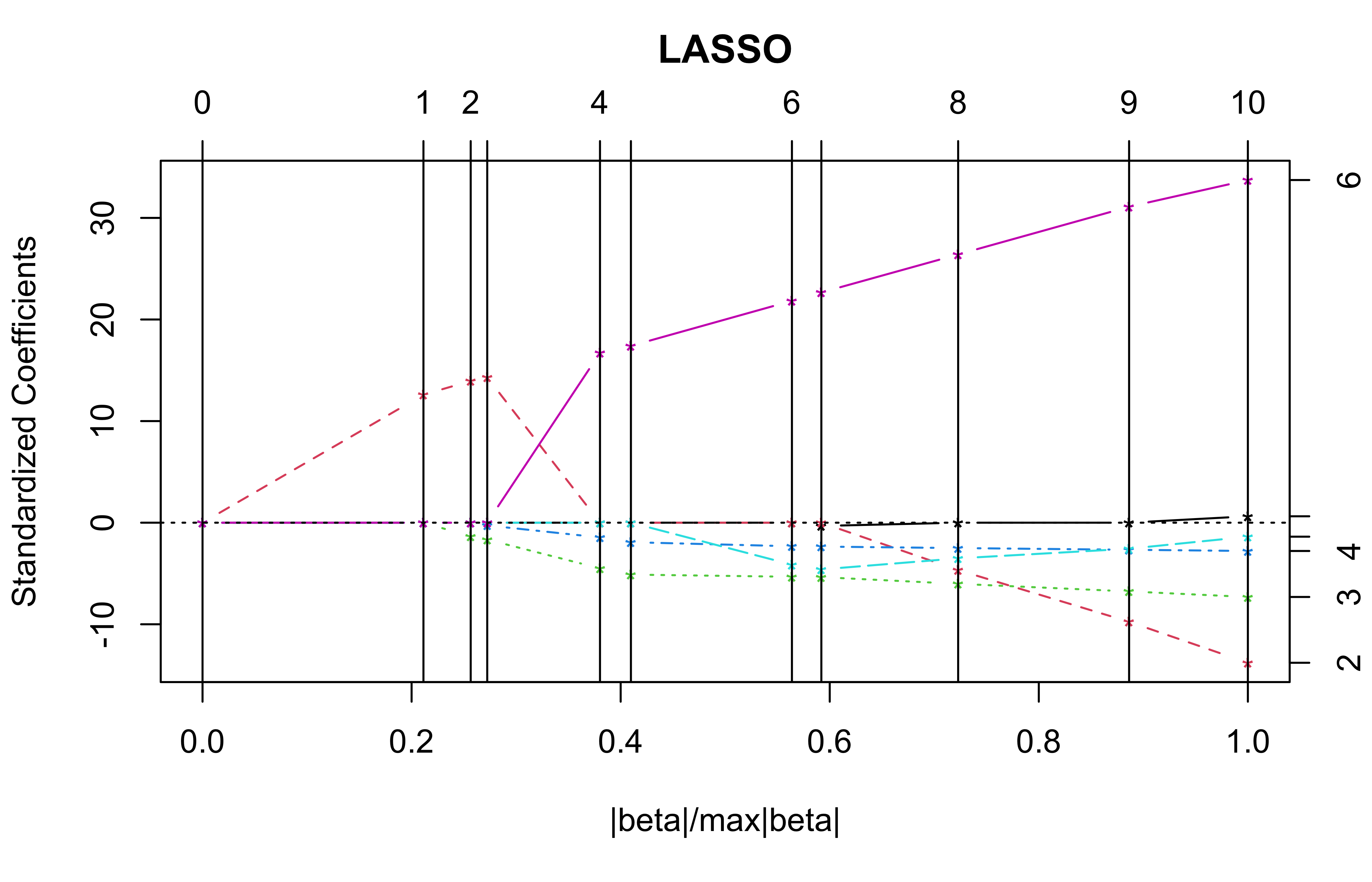
Coefficients

round(coef(longley.lars),4)

      GNP.deflator     GNP Unemployed Armed.Forces Population   Year
 [1,]       0.0000  0.0000     0.0000       0.0000     0.0000 0.0000
 [2,]       0.0000  0.0327     0.0000       0.0000     0.0000 0.0000
 [3,]       0.0000  0.0362    -0.0037       0.0000     0.0000 0.0000
 [4,]       0.0000  0.0372    -0.0046      -0.0010     0.0000 0.0000
 [5,]       0.0000  0.0000    -0.0124      -0.0054     0.0000 0.9068
 [6,]       0.0000  0.0000    -0.0141      -0.0071     0.0000 0.9438
 [7,]       0.0000  0.0000    -0.0147      -0.0086    -0.1534 1.1843
 [8,]      -0.0077  0.0000    -0.0148      -0.0087    -0.1708 1.2289
 [9,]       0.0000 -0.0121    -0.0166      -0.0093    -0.1303 1.4319
[10,]       0.0000 -0.0253    -0.0187      -0.0099    -0.0951 1.6865
[11,]       0.0151 -0.0358    -0.0202      -0.0103    -0.0511 1.8292

Selecting a Solution from the Path

summary(longley.lars)

LARS/LASSO
Call: lars(x = as.matrix(longley[, -7]), y = longley[, 7], type = "lasso")
   Df     Rss        Cp
0   1 185.009 1976.7120
1   2   6.642   59.4712
2   3   3.883   31.7832
3   4   3.468   29.3165
4   5   1.563   10.8183
5   4   1.339    6.4068
6   5   1.024    5.0186
7   6   0.998    6.7388
8   7   0.907    7.7615
9   6   0.847    5.1128
10  7   0.836    7.0000

• For \(p\) predictors, \[C_p = \frac{\textsf{SSE}_p}{s^2} -n + 2p\]

• \(s^2\) is the residual variance from the full model

• \(\textsf{SSE}_p\) is the sum of squared errors for the model with \(p\) predictors (RSS)

• if the model includes all the predictors with non-zero coefficients, then \(C_p \approx p\)

• choose minimum \(C_p \approx p\)

• in practice use Cross-validation or Generalized Cross Validation (GCV) to choose \(\lambda\)

Features and Issues

• Combines shrinkage (like Ridge Regression) with Variable Selection to deal with collinearity

• Can be used for prediction or variable selection

• not invariant under linear transformations of the predictors

• typically no uncertainty estimates for the coefficients or predictions

• ignores uncertainty in the choice of \(\lambda\)

• may overshrink large coefficients

Bayesian LASSO

• Equivalent to finding posterior mode with a Double Laplace Prior \[ \mathop{\mathrm{argmax}}_{\boldsymbol{\beta}} -\frac{\phi}{2} \{ \| \mathbf{Y}_c - \mathbf{X}_s \boldsymbol{\beta}\|^2 + \lambda^* \|\boldsymbol{\beta}\|_1 \} \]

• Park & Casella (JASA 2008) and Hans (Biometrika 2010) propose Bayesian versions of the Lasso \[\begin{eqnarray*} \mathbf{Y}\mid \alpha, \boldsymbol{\beta}, \phi & \sim & \textsf{N}(\mathbf{1}_n \alpha + \mathbf{X}^s \boldsymbol{\beta}^s, \mathbf{I}_n/\phi) \\ \boldsymbol{\beta}\mid \alpha, \phi, \boldsymbol{\tau}& \sim & \textsf{N}(\mathbf{0}, \textsf{diag}(\boldsymbol{\tau}^2)/\phi) \\ \tau_1^2 \ldots, \tau_p^2 \mid \alpha, \phi & \mathrel{\mathop{\sim}\limits^{\rm iid}}& \textsf{Exp}(\lambda^2/2) \\ p(\alpha, \phi) & \propto& 1/\phi \\ \end{eqnarray*}\]

• Generalizes Ridge Priors to allow different prior variances for each coefficient

Double Exponential or Double Laplace Prior

• Marginal distribution of \(\beta_j\) \[\begin{eqnarray*} \boldsymbol{\beta}\mid \alpha, \phi, \boldsymbol{\tau}& \sim & \textsf{N}(\mathbf{0}, \textsf{diag}(\boldsymbol{\tau}^2)/\phi) \\ \tau_1^2 \ldots, \tau_p^2 \mid \alpha, \phi & \mathrel{\mathop{\sim}\limits^{\rm iid}}& \textsf{Exp}(\lambda^2/2) \\ p(\beta_j \mid \phi, \lambda) & = & \int_0^\infty p(\beta_i \mid \phi, \tau^2_j) p(\tau^2_j \mid \phi, \lambda) \, d\tau^2 \\ \end{eqnarray*}\]

• Can show that \(\beta_j \mid \phi, \lambda \mathrel{\mathop{\sim}\limits^{\rm iid}}DE(\lambda \sqrt{\phi})\) \[\int_0^\infty \frac{1}{\sqrt{2 \pi t}} e^{-\frac{1}{2} \phi \frac{\beta^2}{t }} \, \frac{\lambda^2}{2} e^{- \frac{\lambda^2 t}{2}}\, dt = \frac{\lambda \phi^{1/2}}{2} e^{-\lambda \phi^{1/2} |\beta|} \]

• Scale Mixture of Normals (Andrews and Mallows 1974)

Gibbs Sampler

• Integrate out \(\alpha\): \(\alpha \mid \mathbf{Y}, \phi \sim \textsf{N}(\bar{y}, 1/(n \phi)\)
  

• \(\boldsymbol{\beta}\mid \boldsymbol{\tau}, \phi, \lambda, \mathbf{Y}_c \sim \textsf{N}(, )\)
  

• \(\phi \mid \boldsymbol{\tau}, \boldsymbol{\beta}, \lambda, \mathbf{Y}_c \sim \mathbf{G}( , )\)
  

• \(1/\tau_j^2 \mid \boldsymbol{\beta}, \phi, \lambda, \mathbf{Y}\sim \textsf{InvGaussian}( , )\)

• \(X \sim \textsf{InvGaussian}(\mu, \lambda)\) has density \[ f(x) = \sqrt{\frac{\lambda^2}{2 \pi}} x^{-3/2} e^{- \frac{1}{2} \frac{ \lambda^2( x - \mu)^2} {\mu^2 x}} \qquad x > 0 \]

• Homework: Derive the full conditionals for \(\boldsymbol{\beta}^s\), \(\phi\), \(1/\tau^2\)

• see Casella & Park

Horseshoe Priors

Carvalho, Polson & Scott (2010) propose an alternative shrinkage prior \[\begin{align*} \boldsymbol{\beta}\mid \phi & \sim \textsf{N}(\mathbf{0}_p, \frac{\textsf{diag}(\tau^2)}{ \phi }) \\ \tau \mid \lambda & \mathrel{\mathop{\sim}\limits^{\rm iid}}C^+(0, \lambda) \\ \lambda & \sim \textsf{C}^+(0, 1/\phi) \\ p(\alpha, \phi) & \propto 1/\phi \end{align*}\]

• \(C^+(0, \lambda)\) is the half-Cauchy distribution with scale \(\lambda\) \[ p(\tau \mid \lambda) = \frac{2}{\pi} \frac{\lambda}{\lambda^2 + \tau_j^2} \]
• \(\textsf{C}^+(0, 1/\phi)\) is the half-Cauchy distribution with scale \(1/\phi\)

Special Case

In the case \(\lambda = \phi = 1\) and with \(\mathbf{X}^t\mathbf{X}= \mathbf{I}\), \(\mathbf{Y}^* = \mathbf{X}^T\mathbf{Y}\) \[\begin{align*} E[\beta_i \mid \mathbf{Y}] & = \textsf{E}_{\kappa_i \mid \mathbf{Y}}[ \textsf{E}_{\beta_i \mid \kappa_i, \mathbf{Y}}[\beta_i \mid \mathbf{Y}] \\ & = \int_0^1 (1 - \kappa_i) y^*_i p(\kappa_i \mid \mathbf{Y}) \ d\kappa_i \\ & = (1 - \textsf{E}[\kappa \mid y^*_i]) y^*_i \end{align*}\] where \(\kappa_i = 1/(1 + \tau_i^2)\) is the shrinkage factor (like in James-Stein)

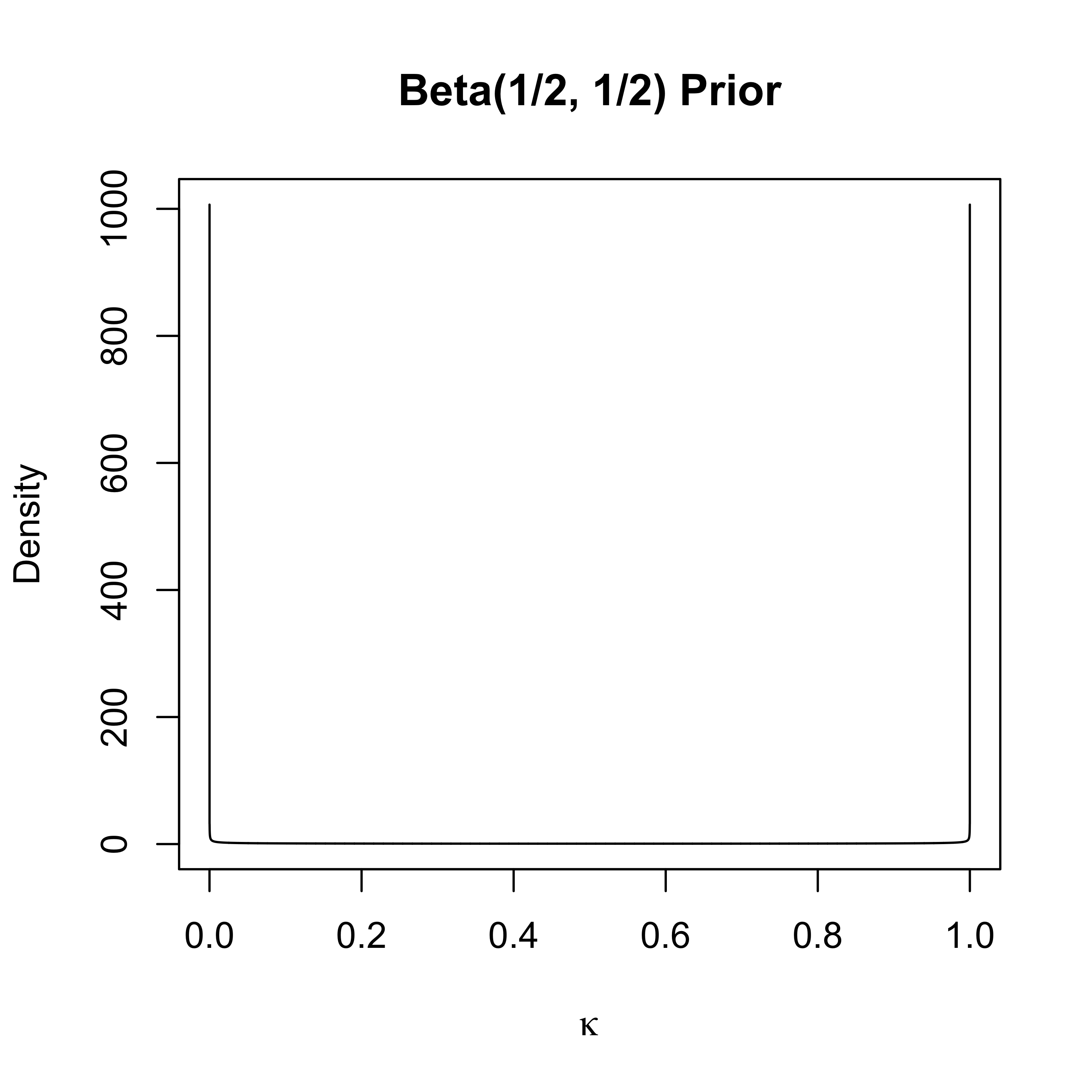
• Half-Cauchy prior induces a Beta(1/2, 1/2) distribution on \(\kappa_i\) a priori (change of variables)

Features and Issues

• the posterior mode also induces shrinkage and variable selection if the mode is at zero

• the posterior mean is a shrinkage estimator (no selection)

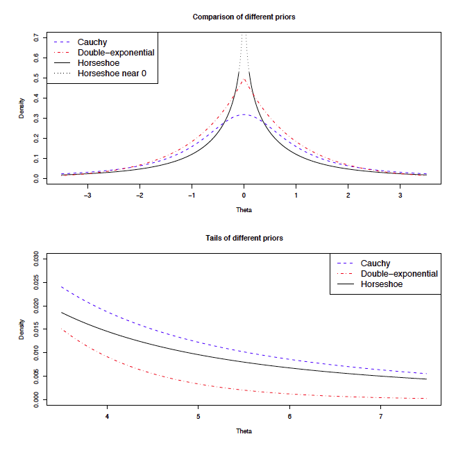
• the tails of the distribution are heavier than the Laplace prior (like a Cauchy distribution) so that there is less shrinkage of large \(|\hat{\boldsymbol{\beta}}|\).

• Desirable in the orthogonal case, where lasso is more like ridge regression (related to bounded influence)

• MCMC is slow to mix using programs like stan but specialized R packages like horseshoe and monomvn::bhsare available

Bounded Influence and Posterior Mean

Posterior mean of \(\beta\) may also be written as \[E[\beta_i \mid y^*_i] = y^*_i + \frac{d} {d y} \log m(y^*_i)\] where \(m(y)\) is the predictive density \(y^*_i\) under the prior (known \(\lambda\))

• HS has Bounded Influence: \[\lim_{|y| \to \infty} \frac{d}{dy} \log m(y) = 0\]

• \(\lim_{|y_i^*| \to \infty} E[\beta_i \mid y^*_i) \to y^*_i\) (the MLE)

• since the MLE \(\to \beta_i^*\) as \(n \to \infty\), the HS is asymptotically consistent

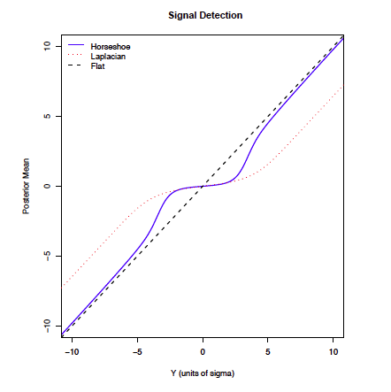
• the DE also has bounded influence, but the bound does not decay to zero in tails so that the posterior mean does not shrink to the MLE

Comparison

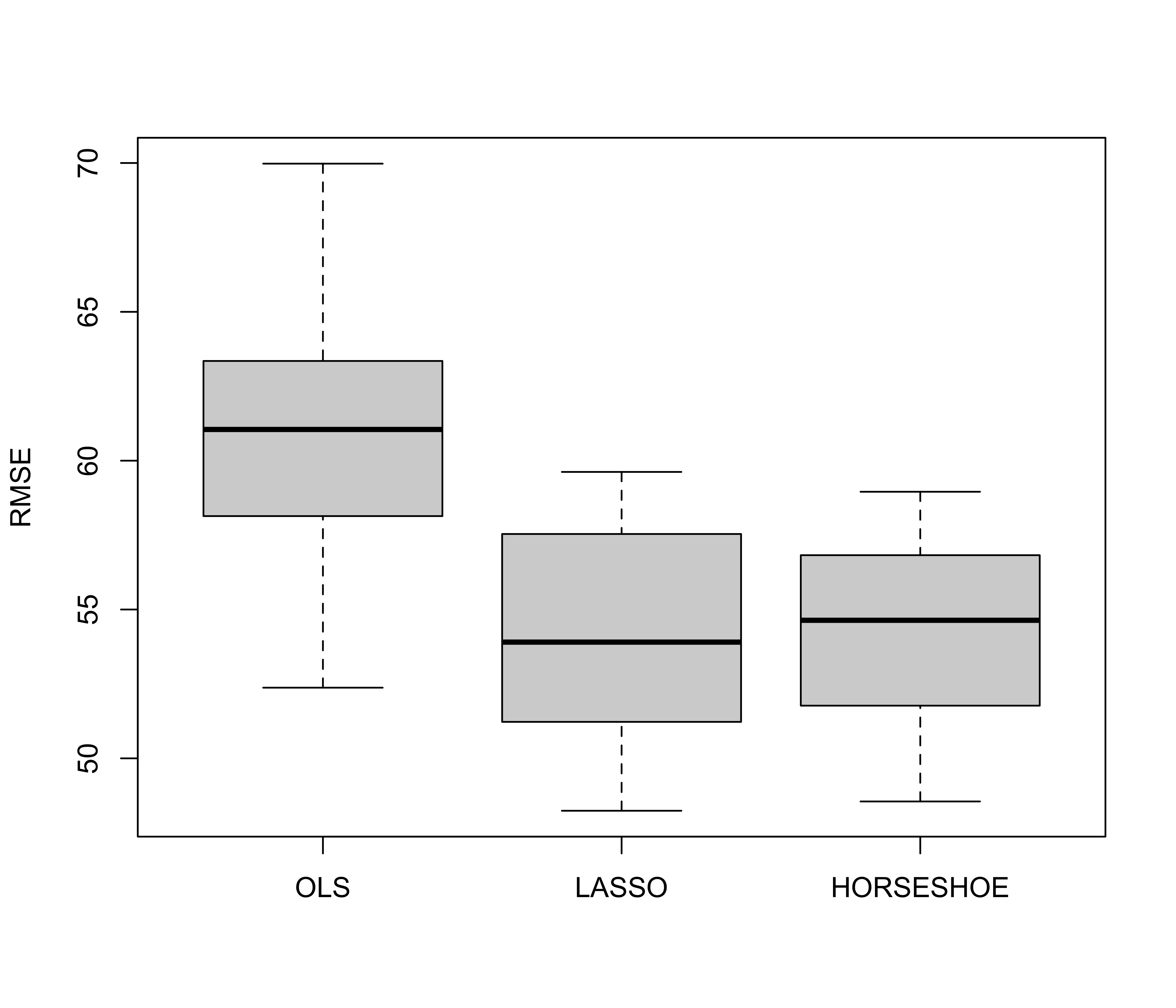
• Diabetes data (from the lars package)

• 64 predictors: 10 main effects, 2-way interactions and quadratic terms

• sample size of 442

• split into training and test sets

• compare MSE for out-of-sample prediction using OLS, lasso and horseshoe priors

• Root MSE for prediction for left out data based on 25 different random splits with 100 test cases

Summary

The literature on shrinkage estimators (with or without selection) is vast

• Elastic Net (Zou & Hastie 2005)
• SCAD (Fan & Li 2001)
• Generalized Double Pareto Prior (Armagan, Dunson & Lee 2013)
• Spike-and-Slab Lasso (Rockova & George 2018)

For Bayes, choice of estimator

• posterior mean (easy via MCMC)
• posterior mode (optimization)
• posterior median (via MCMC)

Properties?

• Fan & Li (JASA 2001) discuss variable selection via non-concave penalties and oracle properties (next time …)