Optimal Shrinkage/Selection and Oracle Properties

STA 721: Lecture 12

Merlise Clyde (clyde@duke.edu)

Duke University

Outline

• Bounded Influence and Posterior Mean

• Shrinkage properties and nonconcave penalties

• conditions for optimal shrinkage and selection . . .

• Readings (see reading link)

  • Tibshirani (JRSS B 1996)
  • Carvalho, Polson & Scott (Biometrika 2010)
  • Armagan, Dunson & Lee (Statistica Sinica 2013)
  • Fan & Li (JASA 2001)

Horseshoe Priors

Carvalho, Polson & Scott (2010) propose an alternative shrinkage prior \[\begin{align*} \boldsymbol{\beta}\mid \phi & \sim \textsf{N}(\mathbf{0}_p, \frac{\textsf{diag}(\tau^2)}{ \phi }) \\ \tau \mid \lambda & \mathrel{\mathop{\sim}\limits^{\rm iid}}C^+(0, \lambda) \\ \lambda & \sim \textsf{C}^+(0, 1/\phi) \\ p(\alpha, \phi) & \propto 1/\phi \end{align*}\]

• \(C^+(0, \lambda)\) is the half-Cauchy distribution with scale \(\lambda\) \[ p(\tau \mid \lambda) = \frac{2}{\pi} \frac{\lambda}{\lambda^2 + \tau_j^2} \]
• \(\textsf{C}^+(0, 1/\phi)\) is the half-Cauchy distribution with scale \(1/\phi\)

Special Case: Orthonormal Regression

In the case \(\lambda = \phi = 1\) and with \(\mathbf{X}^t\mathbf{X}= \mathbf{I}\), \(\mathbf{Y}^* = \mathbf{X}^T\mathbf{Y}\) \[\begin{align*} E[\beta_i \mid \mathbf{Y}] & = \textsf{E}_{\kappa_i \mid \mathbf{Y}}[ \textsf{E}_{\beta_i \mid \kappa_i, \mathbf{Y}}[\beta_i \mid \mathbf{Y}] \\ & = \int_0^1 (1 - \kappa_i) y^*_i p(\kappa_i \mid \mathbf{Y}) \ d\kappa_i \\ & = (1 - \textsf{E}[\kappa \mid y^*_i]) y^*_i \end{align*}\] where \(\kappa_i = 1/(1 + \tau_i^2)\) is the shrinkage factor (like in James-Stein)

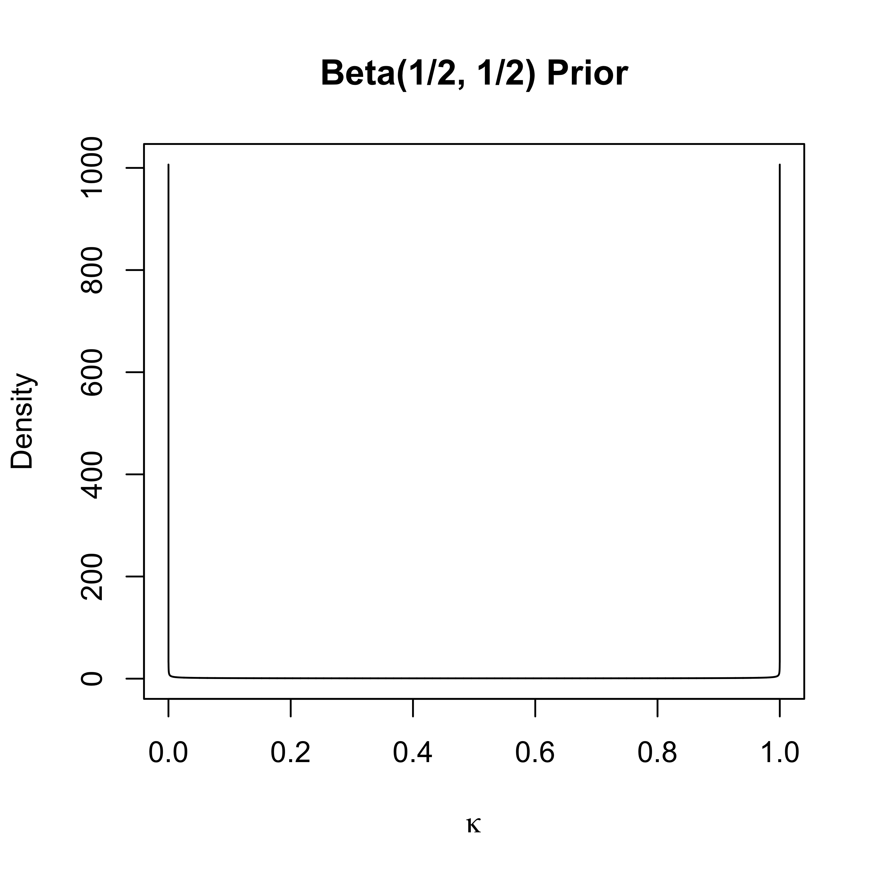
• Half-Cauchy prior induces a Beta(1/2, 1/2) distribution on \(\kappa_i\) a priori (change of variables)

• marginal prior (after integrating out )

Bounded Influence (\(\mathbf{X}^T\mathbf{X}= \mathbf{I}\))

• Posterior mean of \(\beta_i\) may be written as \[E[\beta_i \mid y^*_i] = y^*_i + \frac{d} {d y} \log m(y^*_i)\] where \(m(y)\) is the predictive density \(y^*_i\) under the prior (known \(\lambda\))

• Bounded Influence of the prior (in this setting) means that \[\lim_{|y| \to \infty} \frac{d}{dy} \log m(y) = c\]

• For HS \(\lim_{|y| \to \infty} \frac{d}{dy} \log m(y) = 0\)

• \(\lim_{|y_i^*| \to \infty} E[\beta_i \mid y^*_i) \to y^*_i\) (the MLE)

• unbiasedness for large \(|y_i^*|\)

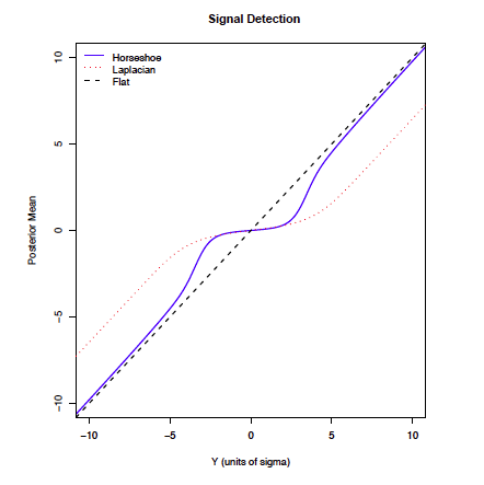
• DE has bounded influence, but bound does not decay to zero in tails so the posterior mean does not shrink to the MLE (bounded away)

Comparison

• Diabetes data (from the lars package)

• 64 predictors: 10 main effects, 2-way interactions and quadratic terms

• sample size of 442

• split into training and test sets

• compare MSE for out-of-sample prediction using OLS, lasso and horseshoe priors

• Root MSE for prediction for left out data based on 25 different random splits with 100 test cases

• both Lasso and Horseshoe much better than OLS

Duality for Modal Estimators

• Model \(Y = \mathbf{X}\boldsymbol{\beta}+ \boldsymbol{\epsilon}\) with \(\mathbf{X}^T\mathbf{X}= \mathbf{I}_p\) and \(\hat{\boldsymbol{\beta}}= \mathbf{X}^T \mathbf{Y}\equiv \mathbf{Y}^*\) (take \(\sigma^2 = 1\))

• Penalized Least Squares \[ \hat{\boldsymbol{\beta}}_j^\lambda = \mathop{\mathrm{argmin}}_{\boldsymbol{\beta}} \ \frac{1}{2}\| \mathbf{Y}- \mathbf{X}\hat{\boldsymbol{\beta}}\|^2 + \frac{1}{2} \sum_j(\beta_j -\hat{\beta}_j)^2 + \sum_j \textsf{pen}_\lambda(\beta_j) \]

• Bayes posterior mode (conditional) with prior \(p(\boldsymbol{\beta}\mid \lambda) = \prod_j p(\beta_j \mid \lambda)\) \[\begin{align*} \hat{\boldsymbol{\beta}}_j^\lambda & =\mathop{\mathrm{argmax}}_{\boldsymbol{\beta}} -\frac{1}{2} \| \mathbf{Y}- \mathbf{X}\hat{\boldsymbol{\beta}}\|^2 - \frac{1}{2} \sum_j(\beta_j -\hat{\beta}_j)^2 + \sum_j \log(p(\beta_j \mid \lambda)) \\ & = \mathop{\mathrm{argmin}}_{\boldsymbol{\beta}} \frac{1}{2}\| \mathbf{Y}- \mathbf{X}\hat{\boldsymbol{\beta}}\|^2 + \frac{1}{2} \sum_j(\beta_j -\hat{\beta}_j)^2 - \sum_j\log(p(\beta_j \mid \lambda)) \\ & = \mathop{\mathrm{argmin}}_{\boldsymbol{\beta}} \frac{1}{2}\| \mathbf{Y}- \mathbf{X}\hat{\boldsymbol{\beta}}\|^2 + \frac{1}{2} \sum_j(\beta_j -\hat{\beta}_j)^2 + \sum_j\textsf{pen}_\lambda(\beta_j) \\ \end{align*}\]

Properties for Modal Estimates

Fan & Li (JASA 2001) discuss variable selection via nonconcave penalties and oracle properties in the context of penalized likelihoods in this setting

• with duality of the negative log prior as their penalty we can extend to Bayesian modal estimates where the prior is a function of \(|\beta_j|\) \[\frac 1 2 \sum(\beta_i - y_i^*)^2 + \frac 1 2 \sum_j(\beta_j - \hat{\beta}_j)^2 + \sum_j \textsf{pen}_\lambda(|\beta_j|)\]

• Requirements on penality

  • Unbiasedness: The resulting estimator is nearly unbiased when the true unknown parameter is large (avoid unnecessary modeling bias).
  • Sparsity: thresholding rule sets small coefficients to 0 (avoid model complexity)
  • Continuity: continuous in the data \(\hat{\beta}_j = y_i^*\) (avoid instability in model prediction)

Conditions for Unbiasedness

To find the optimal estimator take derivative of \(\frac 1 2 \sum_j(\beta_j - \hat{\beta}_j)^2 + \sum_j \textsf{pen}_\lambda(|\beta_j|)\) componentwise and set to zero

• Derivative is \[\begin{align*} \frac{d}{d\,\beta_j} \left\{\frac 1 2 (\beta_j - \hat{\beta}_j)^2 + \textsf{pen}_\lambda(|\beta_j|)\right\} & = (\beta_j - \hat{\beta}_j) + \mathop{\mathrm{sgn}}(\beta_j)\textsf{pen}^\prime_\lambda(|\beta_j|) \\ & = \mathop{\mathrm{sgn}}(\beta_j)\left\{|\beta_j| + \textsf{pen}^\prime_\lambda(|\beta_j|) \right\} - \hat{\beta}_j \end{align*}\]

• setting derivative to zero gives \(\hat{\beta}_j = \mathop{\mathrm{sgn}}(\beta_j)\left\{|\beta_j| + \textsf{pen}^\prime_\lambda(|\beta_j|) \right\}\)

• if \(\lim_{|\beta_j| \to \infty} \textsf{pen}^\prime_\lambda(|\beta|) = 0\) then \(\hat{\beta}_j = \mathop{\mathrm{sgn}}(\beta_j) |\beta_j| = \beta_j\)

• for large \(|\beta_j|\), \(|\hat{\beta}_j|\) is large with high probability

• as MLE is unbiased, the optimal estimator is approximately unbiased for large \(|\beta_j|\)

Conditions for Thresholding & Continuity

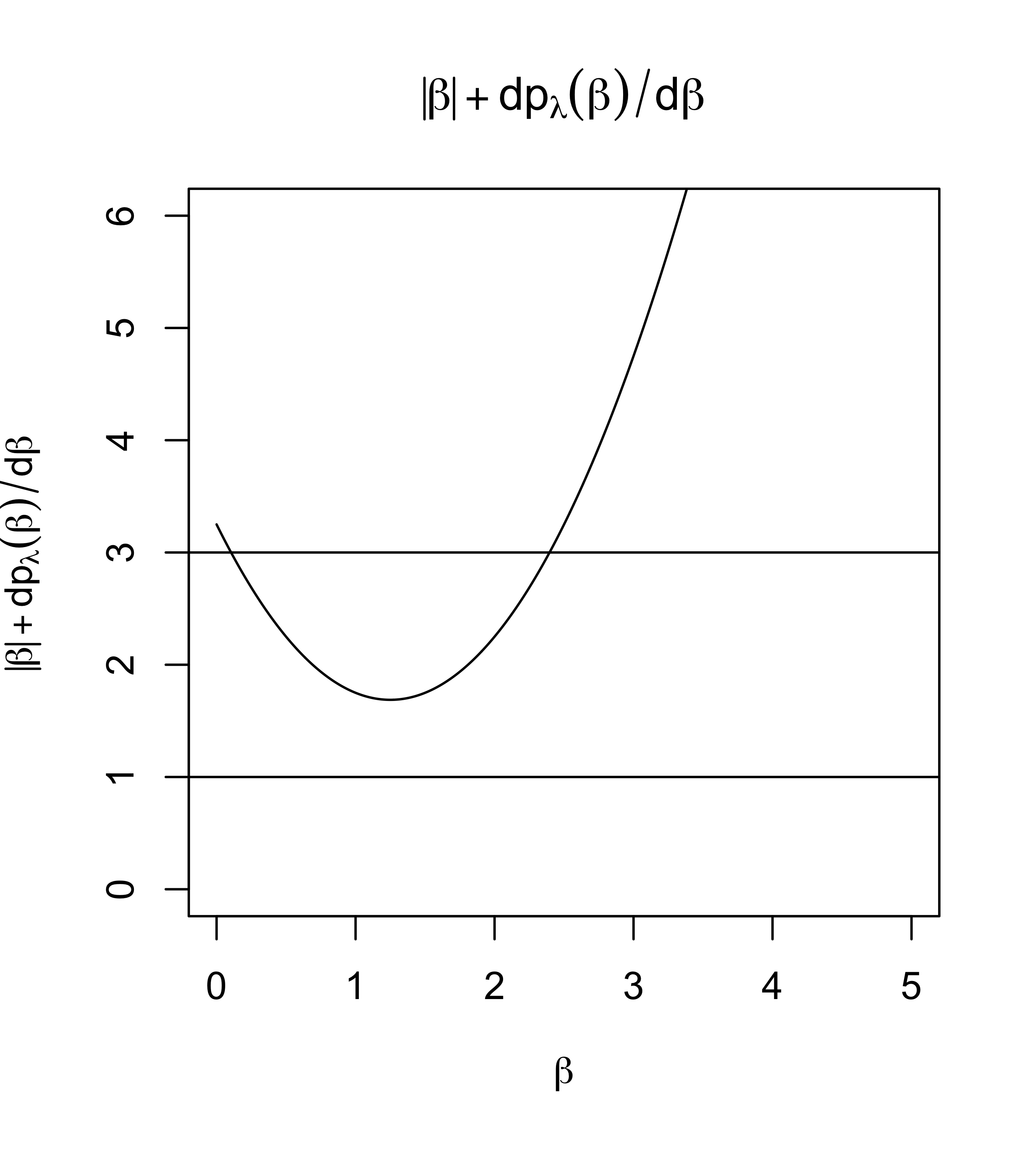
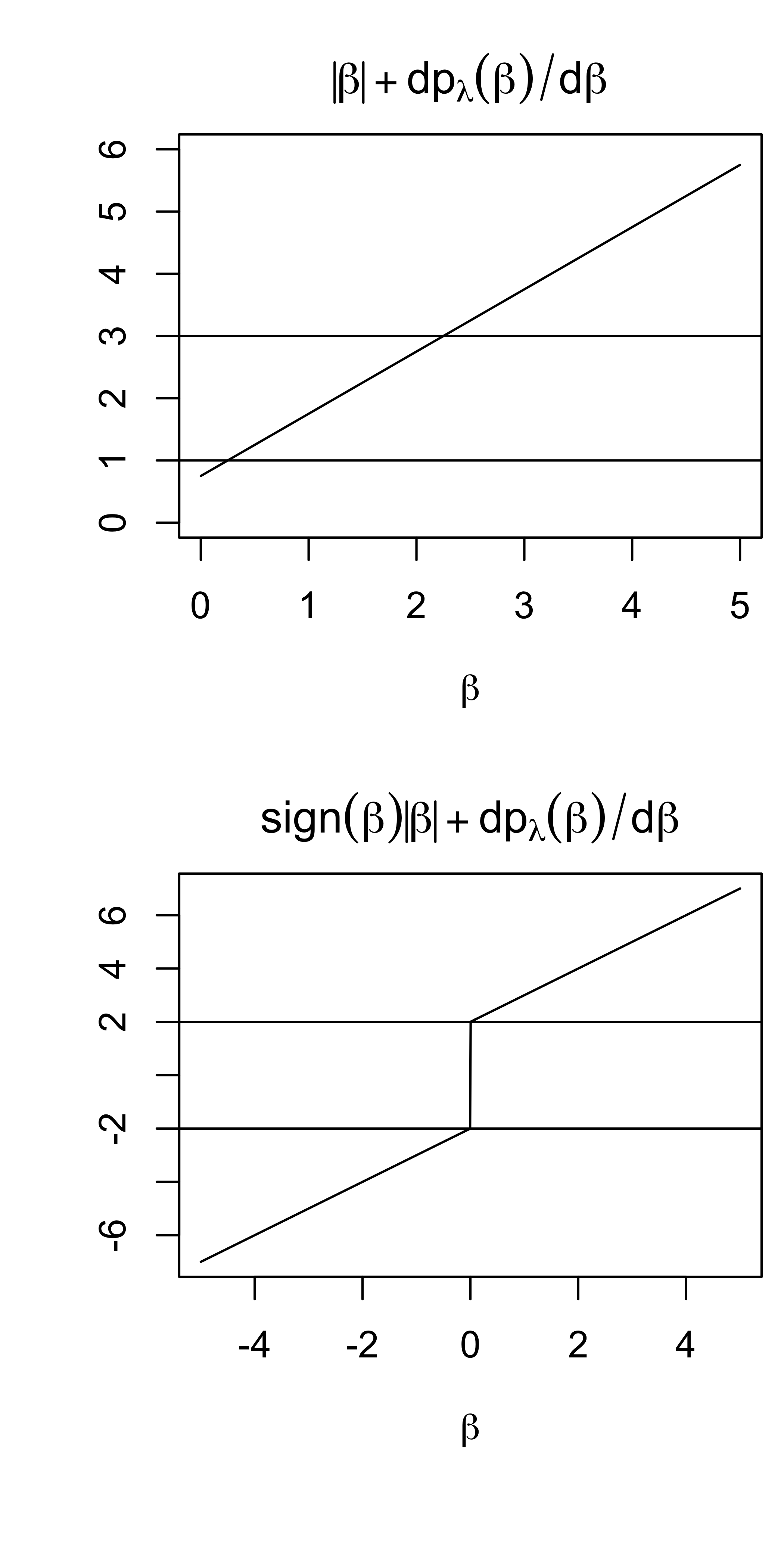
As sufficient condition for a thresholding rule \(\hat{\boldsymbol{\beta}}_j^\lambda = 0\) is if \[0 < \min \left\{ |\beta_j| + \textsf{pen}^\prime_\lambda(|\beta_j|)\right\}\]

• if \(|\hat{\beta}_j| < \min \left\{ |\beta_j| + \textsf{pen}^\prime_\lambda(|\beta_j|) \right\}\) then the derivative is positive for all positive \(\beta_j\) and negative for all negative \(\beta_j\) so \(\hat{\beta}_j^\lambda = 0\) is a local minimum

• if \(|\hat{\beta}_j| > \min \left\{ |\beta_j| + \textsf{pen}^\prime_\lambda(|\beta_j|) \right\}\) multiple crossings (local roots)

• a sufficient and necessary condition for continuity is that the minimum of \(|\beta_j| + \textsf{pen}^\prime_\lambda(|\beta_j|)\) is obtained at zero

Example: Gaussian Prior

• Prior \(\textsf{N}(0, 1/\lambda^2)\)

• Penalty: \(\textsf{pen}_\lambda(|\beta_j|) = \frac{1}{2} \lambda |\beta_j|^2\)

• Unbiasedness: for large \(|\beta_j|\)?

  • Derivative of \(\textsf{pen}_\lambda(|\beta_j|) = \lambda \beta_j = \mathop{\mathrm{sgn}}(\beta_j) \lambda |\beta_j|\)
  • does not go to zero as \(|\beta_j| \to \infty\)
  • No! (bias towards zero)

• not a thresholding rule as \[\min \left\{ |\beta_j| + \textsf{pen}^\prime_\lambda(|\beta_j|)\right\} = (1 + \lambda)|\beta_j|\] is zero

• is continuous as minimum is at zero

Example: Lasso Prior

• Penalty: \(\textsf{pen}_\lambda(|\beta_j|) = \lambda |\beta_j|\)

• Unbiasedness: for large \(|\beta_j|\)?

  • Derivative of \(\textsf{pen}_\lambda(|\beta_j|) = \lambda \mathop{\mathrm{sgn}}(\beta_j)\)
  • does not go to zero as \(|\beta_j| \to \infty\)
  • No! (bias towards zero)

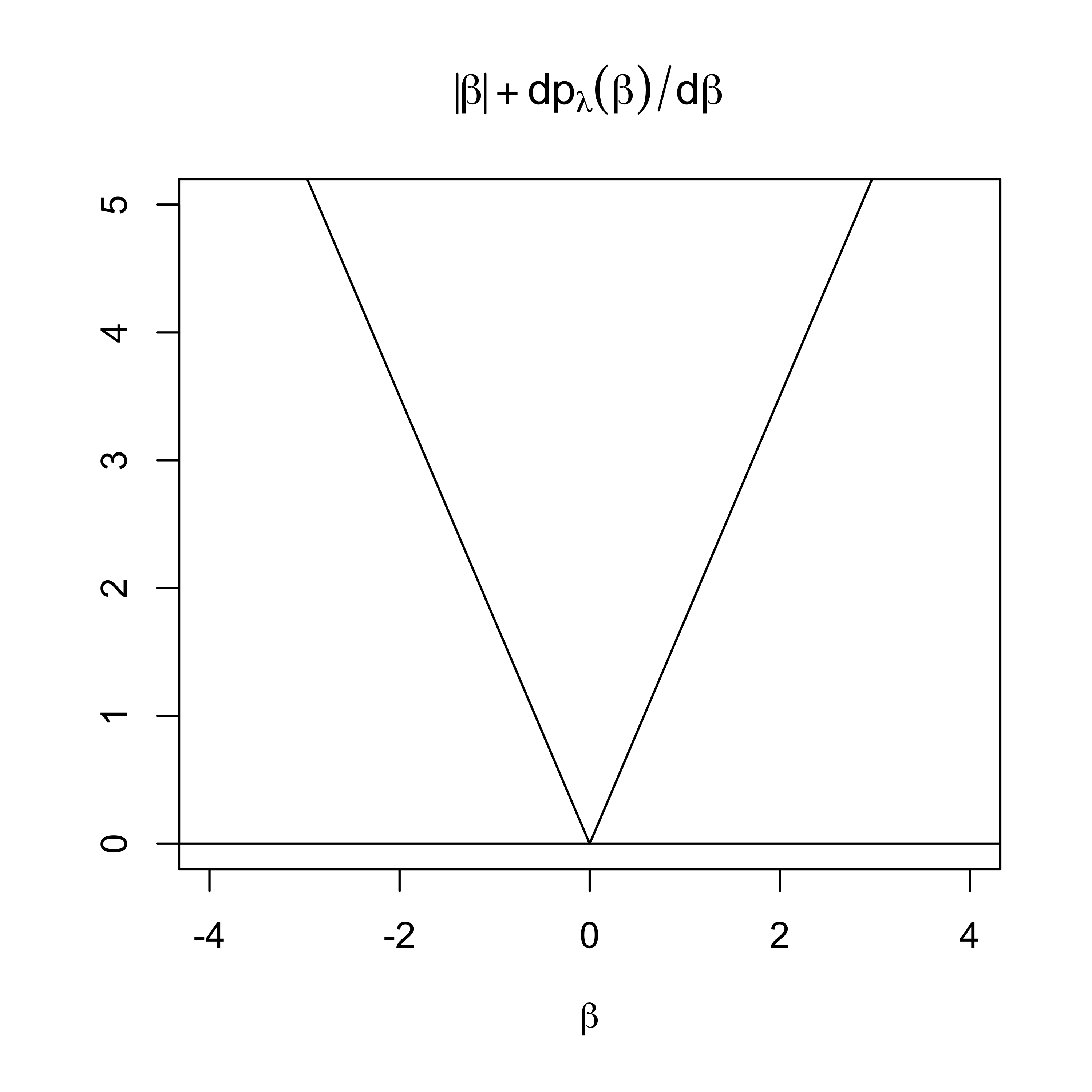
• Is a thresholding rule as \[\min \left\{ |\beta_j| + \textsf{pen}^\prime_\lambda(|\beta_j|)\right\} = (|\beta_j| + \lambda) > 0 \]

• is continuous as minimum is at \(\beta_j = 0\)

Generalized Double Pareto Prior

The Generalized Double Pareto of Armagan, Dunson & Lee (2013)
has a prior density for \(\beta_j\) of the form \[ p(\beta_j \mid \xi, \alpha) = \frac{1}{2 \xi} \left(1 + \frac{\beta_j}{\alpha \xi}\right)^{-(1 + \alpha)} \]

• express as \(\beta_j \mid \xi, \alpha \sim \textsf{GDP}(\xi, \alpha)\)

• Scale mixtures of Normals representation \[\begin{align*} \beta \mid \tau_j & \sim \textsf{N}(0, \tau_j) \\ \tau_j \mid \lambda_j & \sim \textsf{Exp}(\lambda_j^2/2) \\ \lambda_j & \sim \textsf{Gamma}(\alpha, \eta) \\ \beta_j & \sim \textsf{GDP}(\xi = \eta/\alpha, \alpha) \end{align*}\]

• is this a thresholding rule? unbiasedness? continuity?

• for all parameters or are there restrictions?

Choice of Penalty/Prior and Conditions

• Ridge: none
• Lasso: does not satisfy conditions for unbiasedness
• GDP: Can show that Generalized Double Pareto does for some choices of hyperparameters
• Horseshoe: need marginal distribution of \(\beta_j\) for penalty
  • marginal generally not available in closed form
  • can show for a special case where there is an analytic expression for the marginal density (\(\lambda = \phi = 1\)) \[p(\beta) = k \exp(\beta^2/2) E_1(\beta^2/2)\]
• where \(E_n(x) = \int_1^\infty \frac{e^{-xt}}{t^n} dt\) for \(n = 1, 2, \ldots\)
• \(E_n^\prime(x) = -E_{n-1}(x)\) for \(n = 1, 2, \ldots\)

Shrinkage Estimators

The literature on shrinkage estimators (with or without selection) is extensive

• Ridge
• Lasso
• Elastic Net (Zou & Hastie 2005)
• SCAD (Fan & Li 2001)
• Generalized Double Pareto Prior (Armagan, Dunson & Lee 2013)
• Spike-and-Slab Lasso (Rockova & George 2018)

For Bayes, choice of estimator

• posterior mean (easy via MCMC)
• posterior mode (optimization)
• posterior median (via MCMC)

Selection and Uncertainty

• Prior/Posterior do not put any probability on the event \(\beta_j = 0\)

• Uncertainty that the coefficient is zero?

• Selection solved as a post-analysis decision problem

• Selection part of model uncertainty

  • add prior probability that \(\beta_j = 0\)
  • combine with decision problem