Hypothesis Testing

STA 721: Lecture 13

Merlise Clyde (clyde@duke.edu)

Duke University

Outline

Hypothesis Testing:

• The hypothesis of no effects

  • F-tests
  • Null distribution
  • Decision procedure

• Testing submodels

  • Extra sum of squares

Readings:

• Christensen Appendix C, Chapter 3

The Hypothesis of No Effects

Suppose we believe the model \[ {\text{M1}} \quad \quad\mathbf{Y}= \mathbf{X}\boldsymbol{\beta}+ \boldsymbol{\epsilon}\quad \quad \boldsymbol{\epsilon}\sim \textsf{N}(0, \sigma^2 \mathbf{I}_n) \] but hypothesize that there is no effect of the \(\mathbf{X}\) variables on \(\mathbf{Y}\)

• If this were true, then the distribution for \(\mathbf{Y}\) would be \[ \quad \quad \quad \quad \quad {\text{ M0}} \quad \quad \mathbf{Y}= \boldsymbol{\epsilon}\quad \quad \boldsymbol{\epsilon}\sim \textsf{N}(0, \sigma^2 \mathbf{I}_n) \]

• For M1, the distribution of \(\mathbf{Y}\) is a collection of normal distributions with \(\boldsymbol{\mu}\in C(\mathbf{X})\) and Covariance a scalar multiple of the \(\mathbf{I}\)

• the distributions for the data \(\mathbf{Y}\) under M0 is a subset of the distributions under M1 or submodel of M1 with \(\boldsymbol{\mu}= \mathbf{0}\)

• Observations \(\mathbf{Y}\) may give us evidence that supports or rejects our hypothesis that the null model, M0, is true

Goal

Our goals are to

• obtain a numerical summary of the evidence
• come up with a decision-making procedure that decides between M1 and M0,
• (frequentist) control the probability of making a certain type of incorrect decision

Procedure based on the following steps:

1. Test statistic: compute a statistic \(t(\mathbf{Y},\mathbf{X})\), a function of observable data;
2. Null distribution: compare \(t(\mathbf{Y},\mathbf{X})\) to the types of values we would expect if M0 is true
3. Decision rule: accept M0 if \(t(\mathbf{Y},\mathbf{X})\) is in accord with its distribution under M0, otherwise reject the submodel M0

Intuition

If \(\hat{\boldsymbol{\beta}}\approx \boldsymbol{\beta}\) then

• if \(\boldsymbol{\beta}= \mathbf{0}\), then \(\mathbf{X}\hat{\boldsymbol{\beta}}\approx \mathbf{0}\)

• if \(\boldsymbol{\beta}\ne \mathbf{0}\), then \(\mathbf{X}\hat{\boldsymbol{\beta}}\not \approx \mathbf{0}\)

• If the null model M0 is correct, then \(\|\mathbf{X}\hat{\boldsymbol{\beta}}\|^2\) should be small

• If incorrect, \(\|\mathbf{X}\hat{\boldsymbol{\beta}}\|^2\) should be big

• We need to quantify this intuition

Decomposition

\[\begin{align*} \mathbf{X}\hat{\boldsymbol{\beta}}& = \mathbf{P}_{\mathbf{X}} \mathbf{Y}\\ & = \mathbf{X}\boldsymbol{\beta}+ \mathbf{P}\boldsymbol{\epsilon} \end{align*}\]

\[\begin{align*} \|\mathbf{X}\hat{\boldsymbol{\beta}}\|^2 & = (\mathbf{X}\boldsymbol{\beta}+ \mathbf{P}\boldsymbol{\epsilon})^T(\mathbf{X}\boldsymbol{\beta}+ \mathbf{P}\boldsymbol{\epsilon}) \\ & = \boldsymbol{\beta}^T \mathbf{X}^T \mathbf{X}\boldsymbol{\beta}+ 2 \boldsymbol{\beta}^T \mathbf{X}^T \mathbf{P}\boldsymbol{\epsilon}+ \boldsymbol{\epsilon}^T \mathbf{P}\boldsymbol{\epsilon}\\ & = \| \mathbf{X}\boldsymbol{\beta}\|^2 + 2 \boldsymbol{\beta}^T \mathbf{X}^T \boldsymbol{\epsilon}+ \boldsymbol{\epsilon}^T \mathbf{P}\boldsymbol{\epsilon} \end{align*}\]

How big is \(\|\mathbf{X}\hat{\boldsymbol{\beta}}\|^2\) on average? How big do we expect it to be under our two models?

Take expectations:

\[\begin{align*} \textsf{E}[\|\mathbf{X}\hat{\boldsymbol{\beta}}\|^2] & = \|\mathbf{X}\boldsymbol{\beta}\|^2 + \textsf{E}[2 \boldsymbol{\beta}^T \mathbf{X}^T \boldsymbol{\epsilon}] + \textsf{E}[\boldsymbol{\epsilon}^T \mathbf{P}\boldsymbol{\epsilon}] \\ & = \|\mathbf{X}\boldsymbol{\beta}\|^2 + 0 + \sigma^2 \textsf{tr}(\mathbf{P}) = \|\mathbf{X}\boldsymbol{\beta}\|^2 + \sigma^2 p \end{align*}\]

• if \(\boldsymbol{\beta}= \mathbf{0}\), then \(\textsf{E}[\|\mathbf{X}\hat{\boldsymbol{\beta}}\|^2] = \sigma^2 p\)

Comparison

If we knew \(\sigma^2\), then

• if \(\|\mathbf{X}\hat{\boldsymbol{\beta}}\|^2/p \approx \sigma^2\), we might decide M0 would be reasonable

• if \(\|\mathbf{X}\hat{\boldsymbol{\beta}}\|^2/p \gg \sigma^2\), then we might decide M0 is unreasonable

But we do not know \(\sigma^2\)

• if we estimate \(\sigma^2\) by \(s^2 = \frac{\mathbf{Y}^T(\mathbf{I}- \mathbf{P})\mathbf{Y}}{n - p}\), then

  • if \(\|\mathbf{X}\hat{\boldsymbol{\beta}}\|^2/p \approx s^2\), we might decide M0 would be reasonable

  • if \(\|\mathbf{X}\hat{\boldsymbol{\beta}}\|^2/p \gg s^2\), then we might decide M0 is unreasonable

Test Statistic

Note: if the null model M0 is correct (\(\boldsymbol{\beta}= \mathbf{0}\)), then both

• \(\|\mathbf{X}\hat{\boldsymbol{\beta}}\|/p\)
• \(\textsf{SSE}/(n-p) = \frac{\mathbf{Y}^T(\mathbf{I}- \mathbf{P})\mathbf{Y}}{n - p}\)

are unbiased estimates of \(\sigma^2\)

If the null model is not correct, but the linear model M1 is correct, then

• \(s^2\) is still an unbiased estimate of \(\sigma^2\)

• \(\|\mathbf{X}\hat{\boldsymbol{\beta}}\|^2/p\) is expected to be bigger than \(\sigma^2\)

• We can use the ratio of the two quantities to form a test statistic \[t(\mathbf{Y}, \mathbf{X}) = \frac{\|\mathbf{X}\hat{\boldsymbol{\beta}}\|^2/p}{\textsf{SSE}/(n-p)} = \frac{\textsf{RSS}/p}{\textsf{SSE}/(n-p)}\]

• \(\textsf{RSS}\) is the regression or model sum of squares

Distributions under the Null Model M0

• \(\textsf{SSE}\sim \sigma^2 \chi^2_{n-p}\)
• \(\|\mathbf{X}(\hat{\boldsymbol{\beta}}- \boldsymbol{\beta})\|^2 \sim \sigma^2 \chi^2_p\)

so under the null model M0 (\(\boldsymbol{\beta}= \mathbf{0}\)), we have

• \(\textsf{SSE}\sim \sigma^2 \chi^2_{n-p}\)

• \(\|\mathbf{X}\hat{\boldsymbol{\beta}}\|^2 \sim \sigma^2 \chi^2_p\)

• they are statistically independent (why?)

• so the ratio \[\begin{align*} t(\mathbf{Y}, \mathbf{X}) & = \frac{\textsf{RSS}/p}{\textsf{SSE}/(n-p)} = \frac{(\textsf{RSS}/\sigma^2)/p}{(\textsf{SSE}/\sigma^2)/(n-p)} \\ & \mathrel{\mathop{=}\limits^{\rm D}}\frac{\chi^2_p/p}{\chi^2_{n-p}/(n-p)} \quad \text{ is independent of } \sigma^2 \end{align*}\] is independent of \(\sigma^2\)

F Distribution

Definition: F distribution

If \(X_1 \sim \chi^2_{d1}\) and \(X_2 \sim \chi^2_{d2}\) and are independent, then the ratio \[F = \frac{X_1/d1}{X_2/d2}\] has an \(F_{d1, d2}\) distribution with \(d1\) and \(d2\) degrees of freedom.

• \(F(\mathbf{Y}) \equiv t(\mathbf{Y}, \mathbf{X}) = \frac{\textsf{RSS}/p}{\textsf{SSE}/(n-p)}\) has an \(F_{p, n-p}\) distribution under the null model M0

Decision Procedure

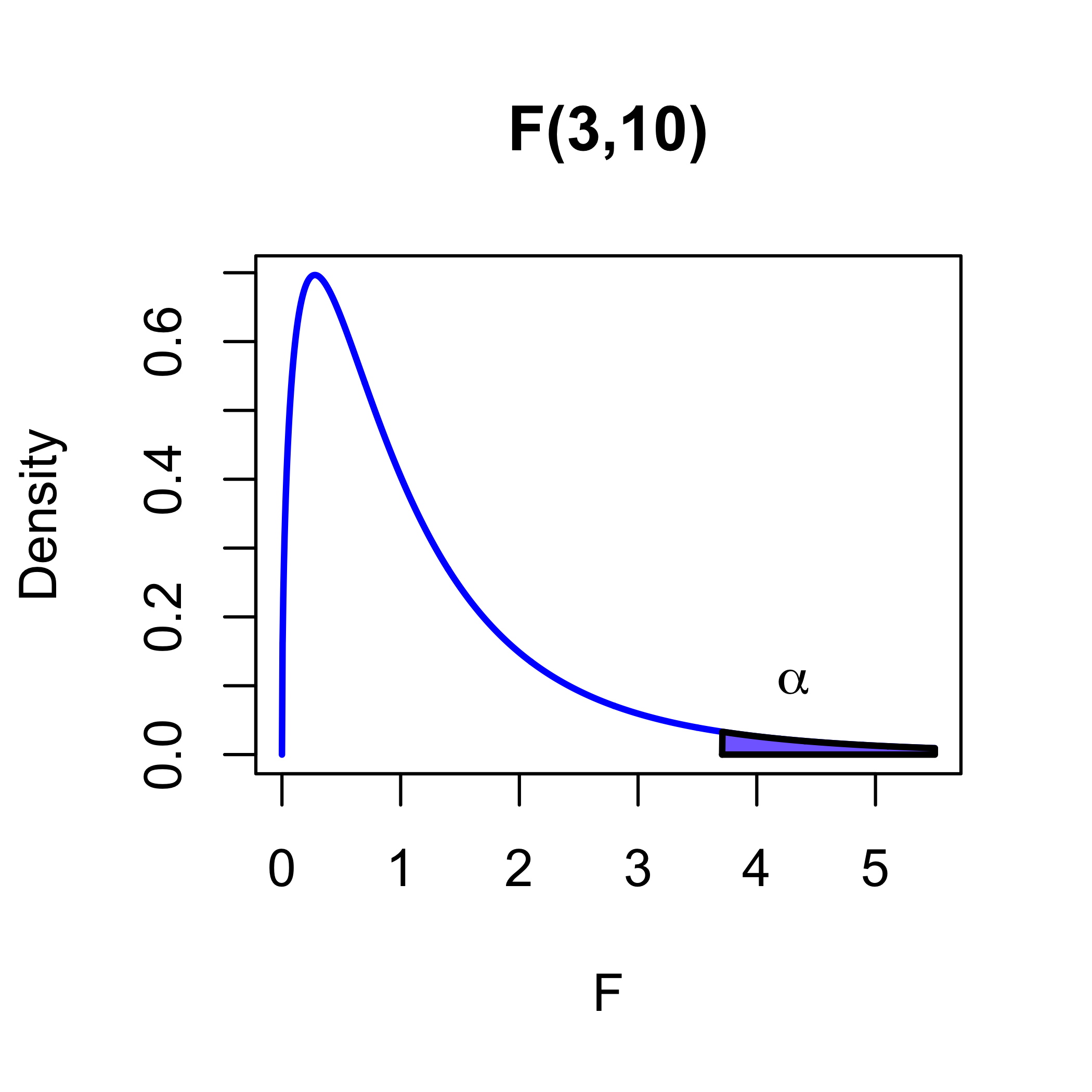
We will accept M0 that \(\boldsymbol{\beta}= \mathbf{0}\) unless \(F(\mathbf{Y})\) is large compared to an \(F_{p,n−p}\) distribution.

• accept M0: \(\boldsymbol{\beta}= \mathbf{0}\) if \(F(\mathbf{Y}) < F_{p,n−p,1−\alpha}\)

• \(F_{p,n−p,1−\alpha}\) is the \(1 − \alpha\) quantile of a \(F_{p,n−p}\)

• reject M0: \(\boldsymbol{\beta}= \mathbf{0}\) if \(F(\mathbf{Y}) > F_{p,n−p,1−\alpha}\)

• the probability that we reject M0 when it is true, is \[\begin{align*} \Pr( \text{ reject M0} & \mid \text{ M0 true})\\ & = \Pr(F(\mathbf{Y}) > F_{p,n−p,1−\alpha} \mid \boldsymbol{\beta}= \mathbf{0}) \\ & = \alpha \end{align*}\]

P-values

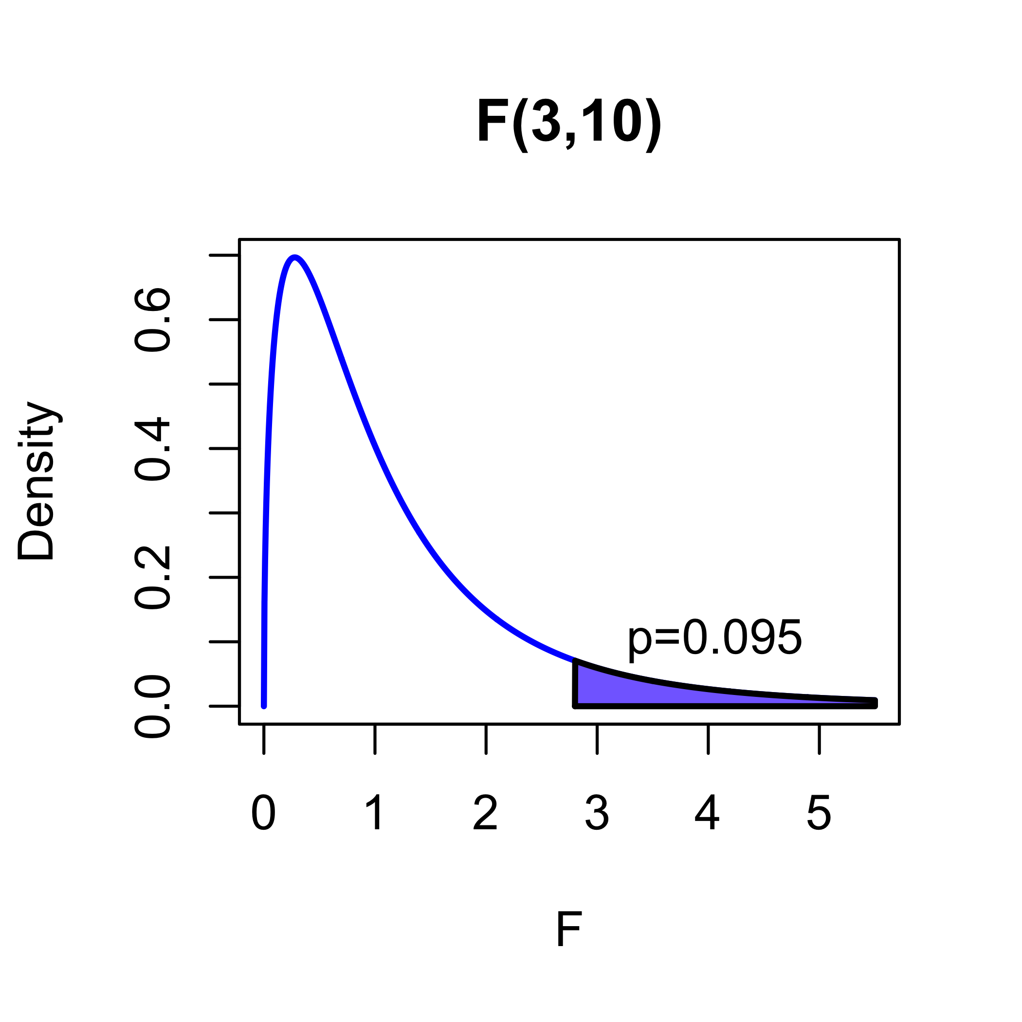
Instead of just declaring that M0 is true or false, statistical analyses report how extreme \(F(\mathbf{Y})\) is compared to its null distribution.

• This is usually reported in terms of the p-value:

  • the value \(p \in(0,1)\) such that \(F(\mathbf{Y})\) is the \((1−p)\) quantile of the \(F_{p,n−p}\) distribution

  • the probability that a random variable \(F \sim F_{p,n−p}\) is larger than the observed value \(F(\mathbf{Y})\), if the null model is true

• it is not the \(\Pr(\text{M0 is true})\) based on the observed data

Testing SubModels

We are usually not interested in testing that all of the coefficients are zero if there is an intercept in the model

• But we can use the same idea to test submodels

• We assume the Gaussian Linear Model \[\quad \quad \quad \quad \quad \quad \quad \quad M1 \quad \mathbf{Y}∼ \textsf{N}(\mathbf{W}\boldsymbol{\alpha}+ \mathbf{X}\boldsymbol{\beta}, \sigma^2\mathbf{I}) \equiv \textsf{N}(\mathbf{Z}\boldsymbol{\theta}, \sigma^2\mathbf{I})\] where \(\mathbf{W}\) is \(n \times q\), \(\mathbf{X}\) is \(n \times p\), \(\mathbf{Z}= [\mathbf{W}\mathbf{X}]\),

• We wish to evaluate the hypothesis \(\boldsymbol{\beta}= \mathbf{0}\)

• equivalent to comparing M1 to M0: \[M0 \quad \mathbf{Y}∼ \textsf{N}(\mathbf{W}\boldsymbol{\alpha}, \sigma^2\mathbf{I})\]

Intuition

Devise a test statistic and procedure by

• fitting the full model M1 \(\mathbf{Y}\sim \textsf{N}(\mathbf{W}\boldsymbol{\alpha}+ \mathbf{X}\boldsymbol{\beta}, \sigma^2\mathbf{I})\)

• fitting the reduced/null model M0 \(\mathbf{Y}\sim \textsf{N}(\mathbf{W}\boldsymbol{\alpha}, \sigma^2\mathbf{I})\)

• accept M0 if the null model fits about as well as the full model

• reject M0 if the null model fits much worse than the full model

• measure fit through \(\textsf{SSE}_{M0}\) and \(\textsf{SSE}_{M1}\) \[\begin{align*} \textsf{SSE}_{M1} & = \min_{\boldsymbol{\alpha}, \boldsymbol{\beta}} \|\mathbf{Y}- (\mathbf{W}\boldsymbol{\alpha}+ \mathbf{X}\boldsymbol{\beta})\|^2 \\ & = \min_{\boldsymbol{\theta}} \|\mathbf{Y}- \mathbf{Z}\boldsymbol{\theta}\|^2 = \mathbf{Y}^T(\mathbf{I}- \mathbf{P}_{\mathbf{Z}})\mathbf{Y}\\ \textsf{SSE}_{M0} & = \min_{\boldsymbol{\alpha}} \|\mathbf{Y}- \mathbf{W}\boldsymbol{\alpha}\|^2 = \mathbf{Y}^T(\mathbf{I}- \mathbf{P}_{\mathbf{W}})\mathbf{Y}\\ \end{align*}\]

Extra Sum of Squares

Approach 1: accept/choose the null model if \(\textsf{SSE}_{M0} < \textsf{SSE}_{M1}\), and choose the full model if \(\textsf{SSE}_{M1} < \textsf{SSE}_{M0}\).

• but \(\textsf{SSE}_{M1}\) is always less than \(\textsf{SSE}_{M0}\)

Approach 2: instead reject M1 \(\boldsymbol{\beta}= \mathbf{0}\) if \(\textsf{SSE}_{M0}\) is much bigger than \(\textsf{SSE}_{M1}\).

• Specifically, reject M1 \(\boldsymbol{\beta}= \mathbf{0}\) if \(\textsf{SSE}_{M0} - \textsf{SSE}_{M1}\) is much bigger than what we would expect if the null hypothesis M0 were true.

Need:

• the null distribution of \(\textsf{SSE}_{M0}\)
• the null distribution of \(\textsf{SSE}_{M1}\)
• the null distribution of their difference \(\textsf{SSE}_{M0} - \textsf{SSE}_{M1}\)

Distributions

Distribution under the full model M1 \[ \textsf{SSE}_{M1} = \mathbf{Y}^T(\mathbf{I}- \mathbf{P}_{\mathbf{Z}})\mathbf{Y}\sim \sigma^2 \chi^2_{n - q - p}\]

• true whether or not \(\boldsymbol{\beta}= \mathbf{0}\)
• \(\textsf{E}[\textsf{SSE}_{M1}] = E[\mathbf{Y}^T(\mathbf{I}- \mathbf{P}_{\mathbf{Z}})\mathbf{Y}] = \sigma^2(n - q - p)\)

Distribution under the null model M0 \[\textsf{SSE}_{M0} = \mathbf{Y}^T(\mathbf{I}- \mathbf{P}_{\mathbf{W}})\mathbf{Y}\sim \sigma^2 \chi^2_{n - q}\]

• true if \(\boldsymbol{\beta}= \mathbf{0}\)
• \(\textsf{E}[\textsf{SSE}_{M0}] = E[\mathbf{Y}^T(\mathbf{I}- \mathbf{P}_{\mathbf{W}})\mathbf{Y}] = \sigma^2(n - q)\)
• if \(\boldsymbol{\beta}\neq \mathbf{0}\) then \(\textsf{SSE}_{M0}\) has a non-central \(\chi^2_{n-q}\) distribution

Expected Value of \(\textsf{SSE}_{M0}\) under M1

• Rewrite \((\mathbf{I}- \mathbf{P}_{\mathbf{W}})\mathbf{Y}\) under M1: \[\begin{align*} (\mathbf{I}- \mathbf{P}_{\mathbf{W}})\mathbf{Y}& = (\mathbf{I}- \mathbf{P}_{\mathbf{W}})(\mathbf{W}\boldsymbol{\alpha}+ \mathbf{X}\boldsymbol{\beta}+ \boldsymbol{\epsilon}) \\ & = (\mathbf{I}- \mathbf{P}_{\mathbf{W}})\mathbf{X}\boldsymbol{\beta}+ (\mathbf{I}- \mathbf{P}_{\mathbf{W}})\boldsymbol{\epsilon} \end{align*}\]

• compute \(\textsf{E}[\textsf{SSE}_{M0}]\) under M1: \[\begin{align*} \textsf{E}[\mathbf{Y}^T(\mathbf{I}- \mathbf{P}_{\mathbf{W}})\mathbf{Y}] & = \boldsymbol{\beta}^T\mathbf{X}^T(\mathbf{I}- \mathbf{P}_{\mathbf{W}})\mathbf{X}\boldsymbol{\beta}+ \textsf{E}[\boldsymbol{\epsilon}^T(\mathbf{I}- \mathbf{P}_{\mathbf{W}})\boldsymbol{\epsilon}] \\ & = \boldsymbol{\beta}^T\mathbf{X}^T(\mathbf{I}- \mathbf{P}_{\mathbf{W}})\mathbf{X}\boldsymbol{\beta}+ \sigma^2 \textsf{tr}(\mathbf{I}- \mathbf{P}_{\mathbf{W}}) \\ & = \boldsymbol{\beta}^T\mathbf{X}^T(\mathbf{I}- \mathbf{P}_{\mathbf{W}})\mathbf{X}\boldsymbol{\beta}+ \sigma^2(n - q) \end{align*}\]

• under M0, both \(\textsf{SSE}_{M0}/(n-q)\) and \(\textsf{SSE}_{M1}/(n- q - p)\) are unbiased estimates of \(\sigma^2\)

• but does the ratio \(\frac{\textsf{SSE}_{M0}/(n-q)}{\textsf{SSE}_{M1}/(n- q - p)}\) have a F distribution?

Extra Sum of Squares

Rewrite \(\textsf{SSE}_{M0}\): \[\begin{align*} \textsf{SSE}_{M0} & = \mathbf{Y}^T(\mathbf{I}- \mathbf{P}_{\mathbf{W}})\mathbf{Y}\\ & = \mathbf{Y}^T(\mathbf{I}- \mathbf{P}_{\mathbf{Z}} + \mathbf{P}_{\mathbf{Z}} - \mathbf{P}_{\mathbf{W}})\mathbf{Y}\\ & = \mathbf{Y}^T(\mathbf{I}- \mathbf{P}_{\mathbf{Z}})\mathbf{Y}+ \mathbf{Y}^T(\mathbf{P}_{\mathbf{Z}} - \mathbf{P}_{\mathbf{W}})\mathbf{Y}\\ & = \textsf{SSE}_{M1} + \mathbf{Y}^T(\mathbf{P}_{\mathbf{Z}} - \mathbf{P}_{\mathbf{W}})\mathbf{Y} \end{align*}\]

Extra Sum of Squares: \[\textsf{SSE}_{M0} - \textsf{SSE}_{M1} = \mathbf{Y}^T(\mathbf{P}_{\mathbf{Z}} - \mathbf{P}_{\mathbf{W}})\mathbf{Y}\]

• is \(\mathbf{P}_{\mathbf{Z}} - \mathbf{P}_{\mathbf{W}}\) is a projection matrix?
• onto what space? along what space ?
• what is the distribution of \(\textsf{SSE}_{M0} - \textsf{SSE}_{M1}\) under the null model M0? under M1?
• is it independent of \(\textsf{SSE}_{M1}\)?