Outliers and Robust Regression

STA 721: Lecture 20

Merlise Clyde

Duke University

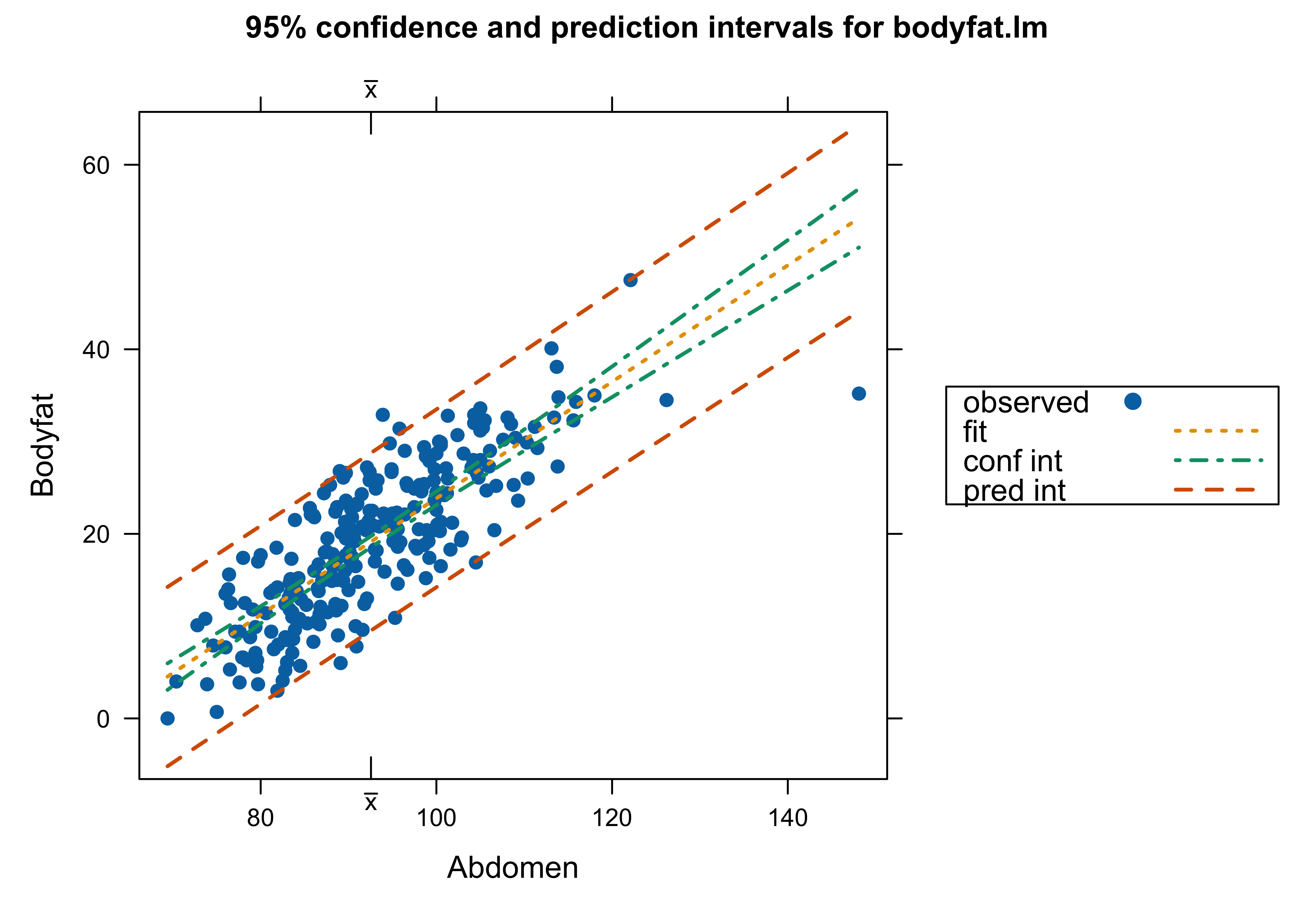
Body Fat Data

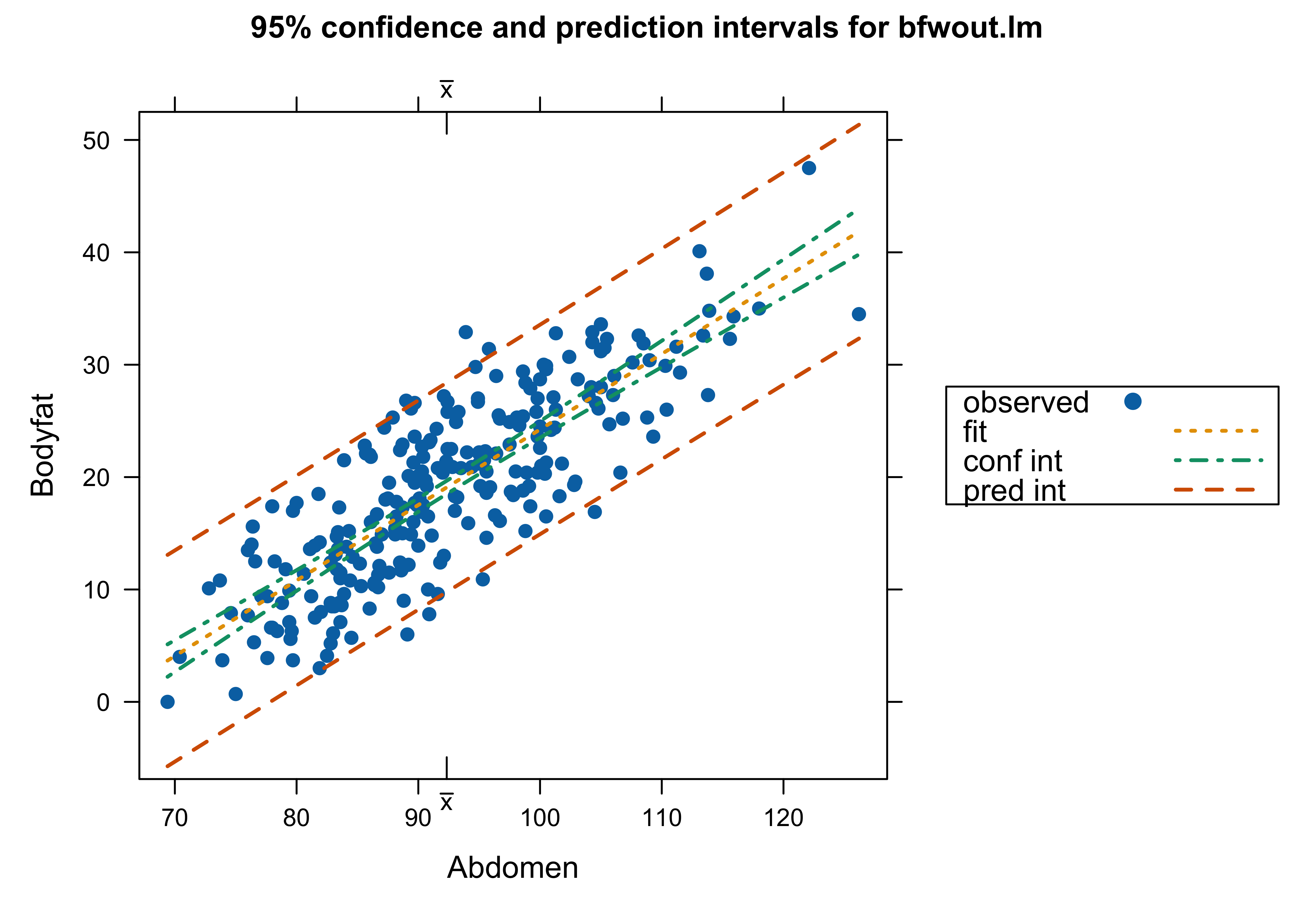
Which analysis do we use? with Case 39 or not – or something different?

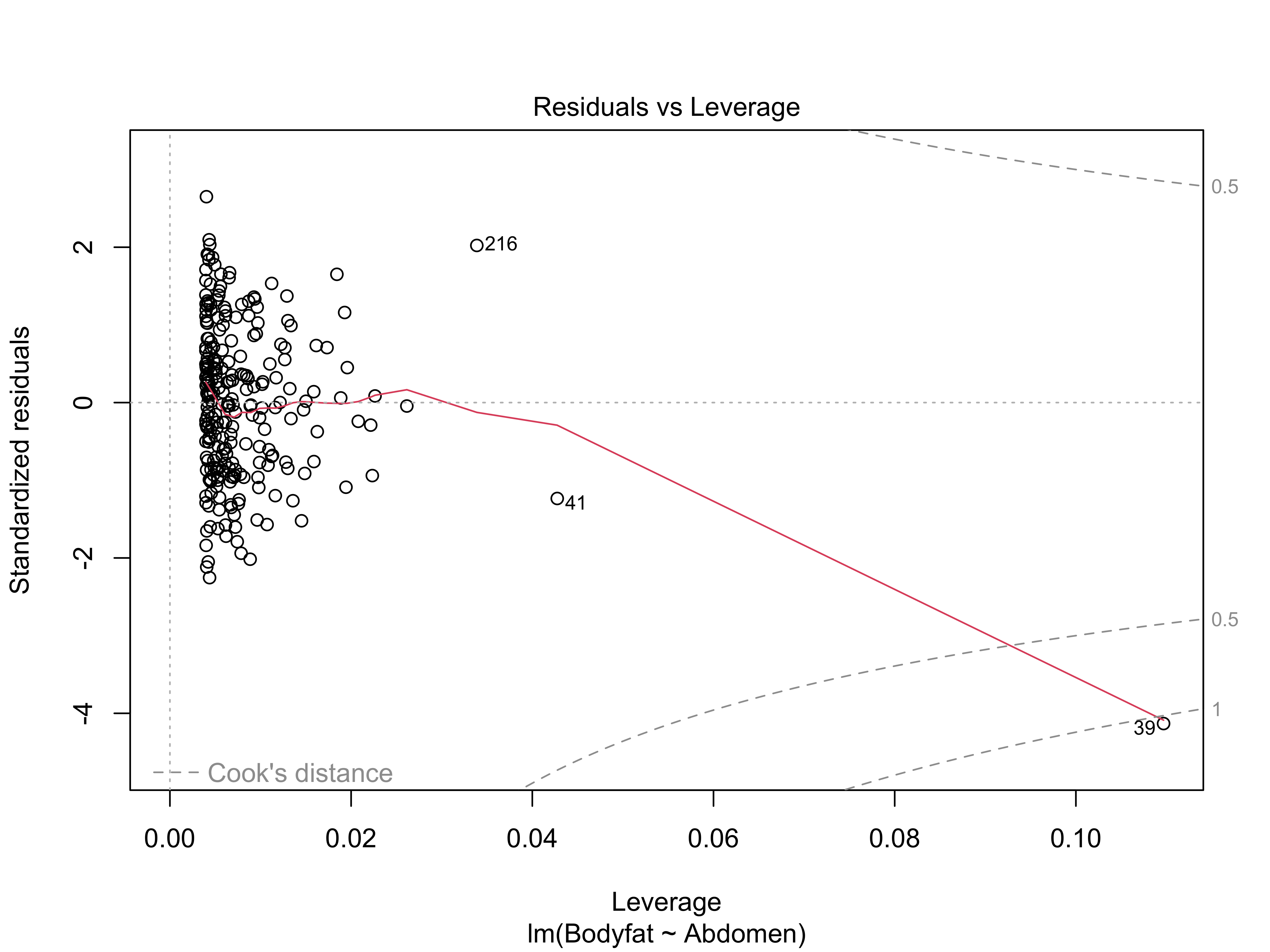
Cook’s Distance

plot(bodyfat.lm, which=5)

Options for Handling Outliers

What are outliers?

• Are there scientific grounds for eliminating the case?

• Test if the case has a different mean than population

• Report results with and without the case

• Model Averaging to Account for Model Uncertainty?

• Full model \(\mathbf{Y}= \mathbf{X}\boldsymbol{\beta}+ \mathbf{I}_n\delta+ \epsilon\)

• \(\delta\) is a \(n \times 1\) vector; \(\boldsymbol{\beta}\) is \(p \times 1\)

• All observations have a potentially different mean!

Outliers in Bayesian Regression

• Hoeting, Madigan and Raftery (in various permutations) consider the problem of simultaneous variable selection and outlier identification

• This is implemented in the package BMA in the function MC3.REG

• This has the advantage that more than 2 points may be considered as outliers at the same time

• The function uses a Markov chain to identify both important variables and potential outliers, but is coded in Fortran so should run reasonably quickly.

• Can also use BAS or other variable selection programs

Model Averaging and Outliers

• Full model \(\mathbf{Y}= \mathbf{X}\boldsymbol{\beta}+ \mathbf{I}_n\delta+ \epsilon\)

• \(\delta\) is a \(n \times 1\) vector; \(\boldsymbol{\beta}\) is \(p \times 1\)

• \(2^n\) submodels \(\gamma_i = 0 \Leftrightarrow \delta_i = 0\)

• If \(\gamma_i = 1\) then case \(i\) has a different mean ``mean shift’’ outliers

Mean Shift \(=\) Variance Inflation

• Model \(\mathbf{Y}= \mathbf{X}\boldsymbol{\beta}+ \mathbf{I}_n\delta+ \epsilon\)

• Prior \[\begin{align} \qquad \delta_i \mid \gamma_i & \sim N(0, V \sigma^2 \gamma_i) \\ \qquad \gamma_i & \sim \textsf{Ber}(\pi) \end{align} \]

• Then \(\epsilon_i\) given \(\sigma^2\) is independent of \(\delta_i\) and \[\epsilon^*_i \equiv \epsilon_i + \delta_i \mid \sigma^2 \left\{ \begin{array}{llc} N(0, \sigma^2) & wp &(1 - \pi) \\ N(0, \sigma^2(1 + V)) & wp & \pi \end{array} \right. \]

• Model \(\mathbf{Y}= \mathbf{X}\boldsymbol{\beta}+ \epsilon^*\) variance inflation

• \(V+1 = K = 7\) in the paper by Hoeting et al. package BMA

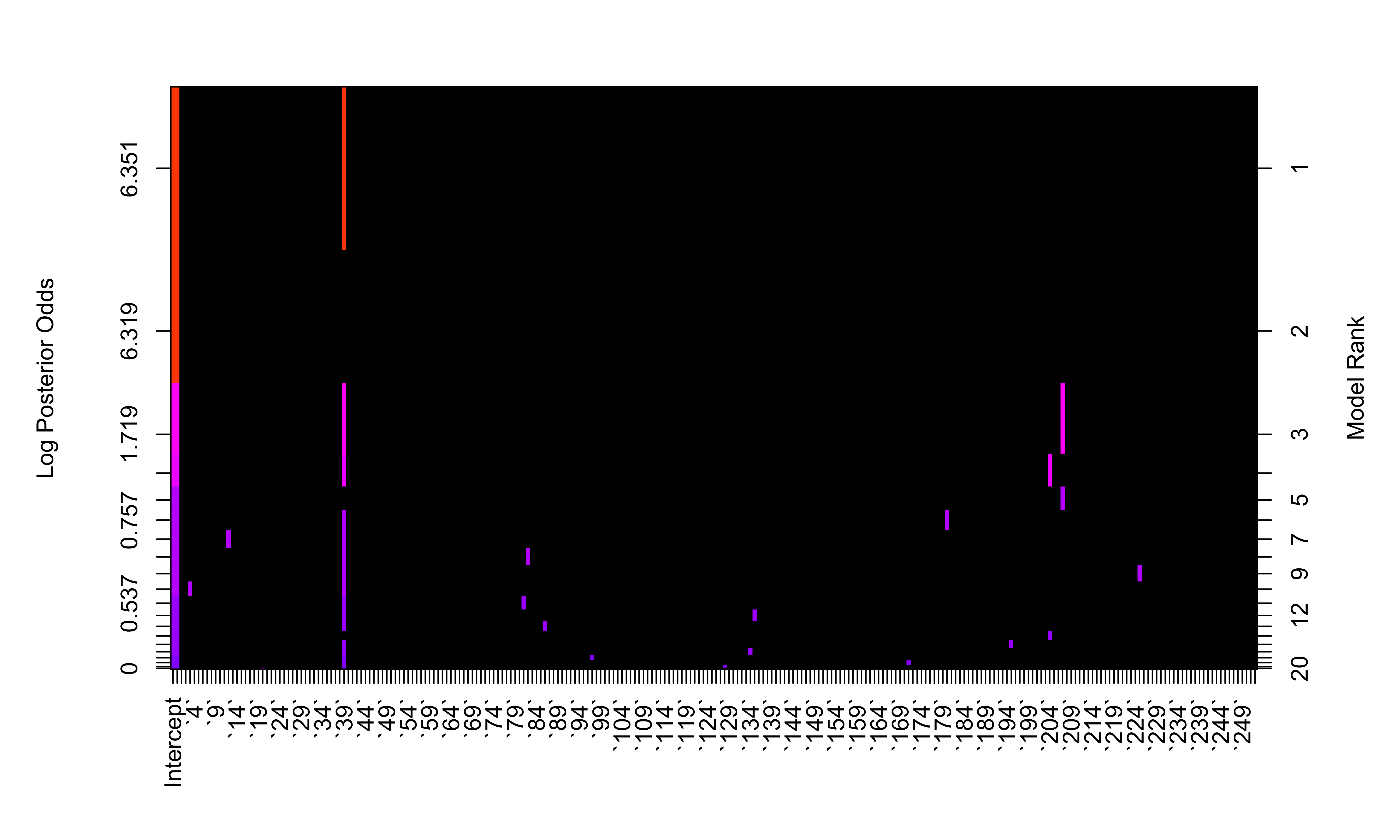
Simultaneous Outlier and Variable Selection

library(BMA)
bodyfat.bma = MC3.REG(all.y = bodyfat$Bodyfat, all.x = as.matrix(bodyfat$Abdomen),
                      num.its = 10000, outliers = TRUE)
summary(bodyfat.bma)

Call:
MC3.REG(all.y = bodyfat$Bodyfat, all.x = as.matrix(bodyfat$Abdomen),     num.its = 10000, outliers = TRUE)

Model parameters: PI = 0.02 K = 7 nu = 2.58 lambda = 0.28 phi = 2.85

  15  models were selected
 Best  5  models (cumulative posterior probability =  0.9939 ): 

           prob     model 1   model 2   model 3   model 4   model 5 
variables                                                           
  all.x    1         x         x         x         x         x      
outliers                                                            
  39       0.94932   x         x         .         x         .      
  204      0.04117   .         .         .         x         .      
  207      0.10427   .         x         .         .         x      
                                                                    
post prob           0.814572  0.095383  0.044490  0.035024  0.004385

BAS with Truncated Prior

bodyfat.w.out = cbind(bodyfat[, c("Bodyfat", "Abdomen")],
                      diag(nrow(bodyfat)))

bodyfat.bas = bas.lm(Bodyfat ~ ., data=bodyfat.w.out, 
                     prior="hyper-g-n", a=3, method="MCMC",
                     MCMC.it=2^18, 
                     modelprior=tr.beta.binomial(1,254, 50))

Change Error Assumptions

Use a Student-t error model \[\begin{eqnarray*} Y_i & \mathrel{\mathop{\sim}\limits^{\rm ind}}& t(\nu, \alpha + \beta x_i, 1/\phi) \\ L(\alpha, \beta,\phi) & \propto & \prod_{i = 1}^n \phi^{1/2} \left(1 + \frac{\phi (y_i - \alpha - \beta x_i)^2}{\nu}\right)^{-\frac{(\nu + 1)}{2}} \end{eqnarray*}\]

• Use Prior \(p(\alpha, \beta, \phi) \propto 1/\phi\)

• Posterior distribution \[ p(\alpha, \beta, \phi \mid Y) \propto \phi^{n/2 - 1} \prod_{i = 1}^n \left(1 + \frac{\phi (y_i - \alpha - \beta x_i)^2}{\nu}\right)^{-\frac{(\nu + 1)}{2}}\]

Bounded Influence

• Treat \(\sigma^2\) as given, then influence of individual observations on the posterior distribution of \(\boldsymbol{\beta}\) in the model where \(\textsf{E}[\mathbf{Y}_i] = \mathbf{x}_i^T\boldsymbol{\beta}\) is investigated through the score function: \[ \frac{d} {d \boldsymbol{\beta}} \log p (\boldsymbol{\beta}\mid \mathbf{Y}) = \frac{d} {d \boldsymbol{\beta}} \log p(\boldsymbol{\beta}) + \sum_{i = 1}^n \mathbf{x}_i g(y_i - \mathbf{x}^T_i \boldsymbol{\beta}) \]

• influence function of the error distribution (unimodal, continuous, differentiable, symmetric) \[ g(\boldsymbol{\epsilon}) = - \frac{d} {d \boldsymbol{\epsilon}} \log p(\boldsymbol{\epsilon}) \]

• An outlying observation \(y_j\) is accommodated if the posterior distribution for \(p(\boldsymbol{\beta}\mid \mathbf{Y}\) converges to \(p(\boldsymbol{\beta}\mid \mathbf{Y}_{(i)})\) for all \(\boldsymbol{\beta}\) as \(|\mathbf{Y}_i| \to \infty\).

• Requires error models with influence functions that go to zero such as the Student \(t\) (O’Hagan, 1979, West 1984, Hamura 2023)

Choice of df for Student-\(t\)

Investigate the Score function \[ \frac{d} {d \boldsymbol{\beta}} \log p (\boldsymbol{\beta}\mid \mathbf{Y}) = \frac{d} {d \boldsymbol{\beta}} \log p(\boldsymbol{\beta}) + \sum_{i = 1}^n \mathbf{x}_i g(y_i - \mathbf{x}^T_i \boldsymbol{\beta}) \]

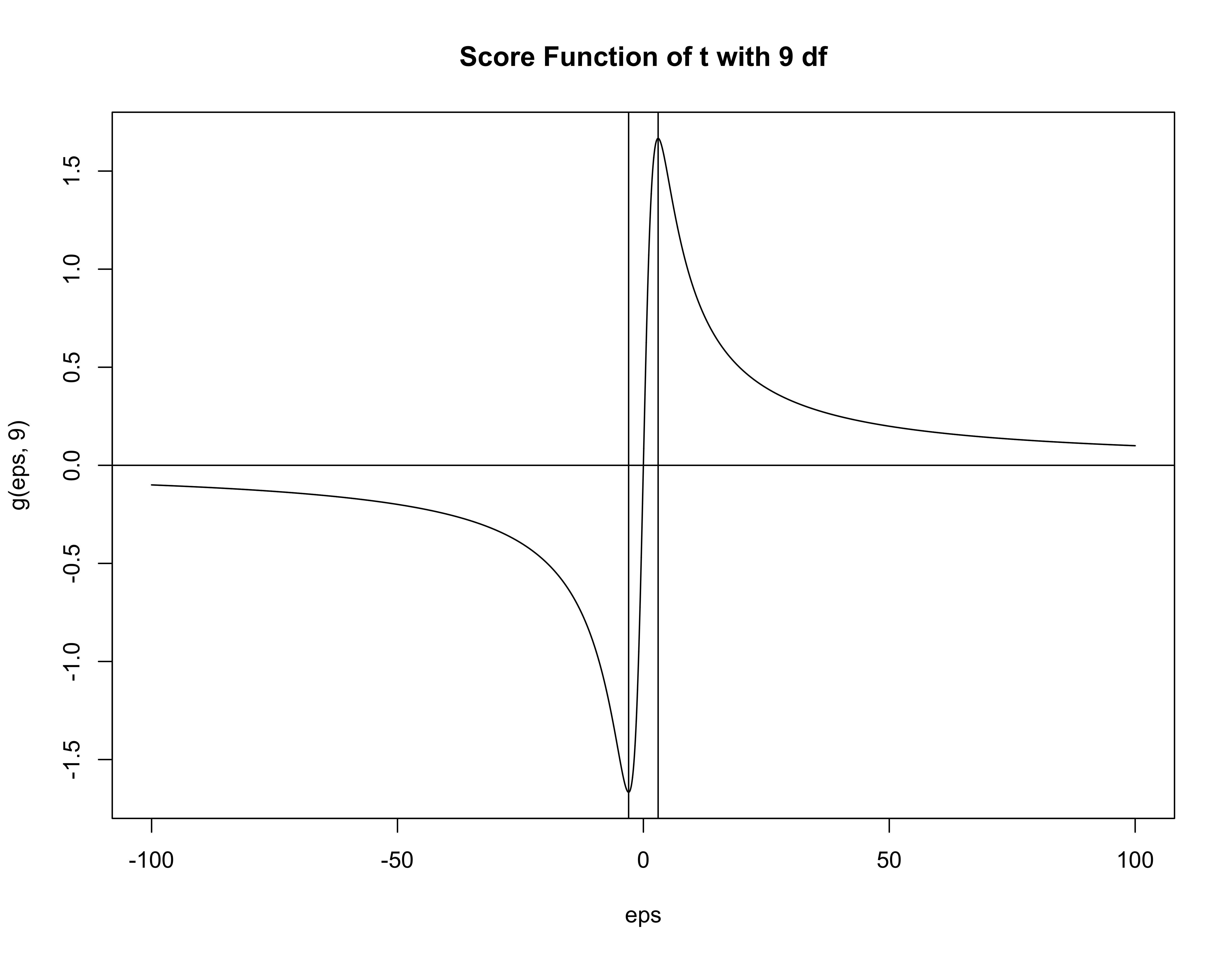
• Score function for \(t\) with \(\alpha\) degrees of freedom has turning points at \(\pm \sqrt{\alpha}\)

• \(g'(\boldsymbol{\epsilon})\) is negative when \(\boldsymbol{\epsilon}^2 > \alpha\) (standardized errors)

• Contribution of observation to information matrix is negative and the observation is doubtful

• Suggest taking \(\alpha = 8\) or \(\alpha = 9\) to reject errors larger than \(\sqrt{8}\) or \(3\) sd.

Scale-Mixtures of Normal Representation

• Latent Variable Model \[\begin{eqnarray*} Y_i \mid \alpha, \beta, \phi, \lambda & \mathrel{\mathop{\sim}\limits^{\rm ind}}& N(\alpha + \beta x_i, \frac{1}{\phi \lambda_i}) \\ \lambda_i & \mathrel{\mathop{\sim}\limits^{\rm iid}}& G(\nu/2, \nu/2) \\ p(\alpha, \beta, \phi) & \propto & 1/\phi \end{eqnarray*}\]

• Joint Posterior Distribution: \[\begin{eqnarray*} p((\alpha, \beta, \phi, \lambda_1, \ldots, \lambda_n \mid Y) \propto \, & & \phi^{n/2} \exp\left\{ - \frac{\phi}{2} \sum \lambda_i(y_i - \alpha - \beta x_i)^2 \right\} \times \\ & & \phi^{-1} \\ & &\prod_{i=1}^n \lambda_i^{\nu/2 - 1} \exp(- \lambda_i \nu/2) \end{eqnarray*}\]

• Integrate out ``latent’’ \(\lambda\)’s to obtain marginal \(t\) distribution

JAGS - Just Another Gibbs Sampler

rr.model = function() {
  df <- 9
  for (i in 1:n) {
    mu[i] <- alpha0 + alpha1*(X[i] - Xbar)
    lambda[i] ~ dgamma(df/2, df/2)
    prec[i] <- phi*lambda[i]
    Y[i] ~ dnorm(mu[i], prec[i])
  }
  phi ~ dgamma(1.0E-6, 1.0E-6)
  alpha0 ~ dnorm(0, 1.0E-6)
  alpha1 ~ dnorm(0,1.0E-6)
  beta0 <- alpha0 - alpha1*Xbar  # transform back
  beta1 <- alpha1
  sigma <- pow(phi, -.5)
  mu34 <- beta0 + beta1*2.54*34  #mean for a man w/ a 34 in waist
  y34 ~ dt(mu34,phi, df)   # integrate out lambda_34 
}

Warning! Normals and Student-t are parameterized in terms of precisions!

What output to Save?

The parameters to be monitored and returned to R are specified with the variable parameters

parameters = c("beta0", "beta1", "sigma", "mu34", "y34", "lambda[39]")

• Use of <- for assignment for parameters that calculated from the other parameters. (See R-code for definitions of these parameters.)

• mu34 and y34 are the mean functions and predictions for a man with a 34in waist.

• lambda[39] saves only the 39th case of \(\lambda\)

• To save a whole vector (for example all lambdas, just give the vector name)

Running JAGS from R

Install jags from sourceforge

library(R2jags)

# Create a data list with inputs for Winpost/Jags

bf.data = list(Y = bodyfat$Bodyfat, X=bodyfat$Abdomen)
bf.data$n = length(bf.data$Y)
bf.data$Xbar = mean(bf.data$X)

# run jags
bf.sim = jags(bf.data, inits=NULL, par=parameters,
              model=rr.model, n.chains=2, n.iter=20000)

# create an MCMC object 
library(coda)
bf.post = as.mcmc(bf.sim$BUGSoutput$sims.matrix)  

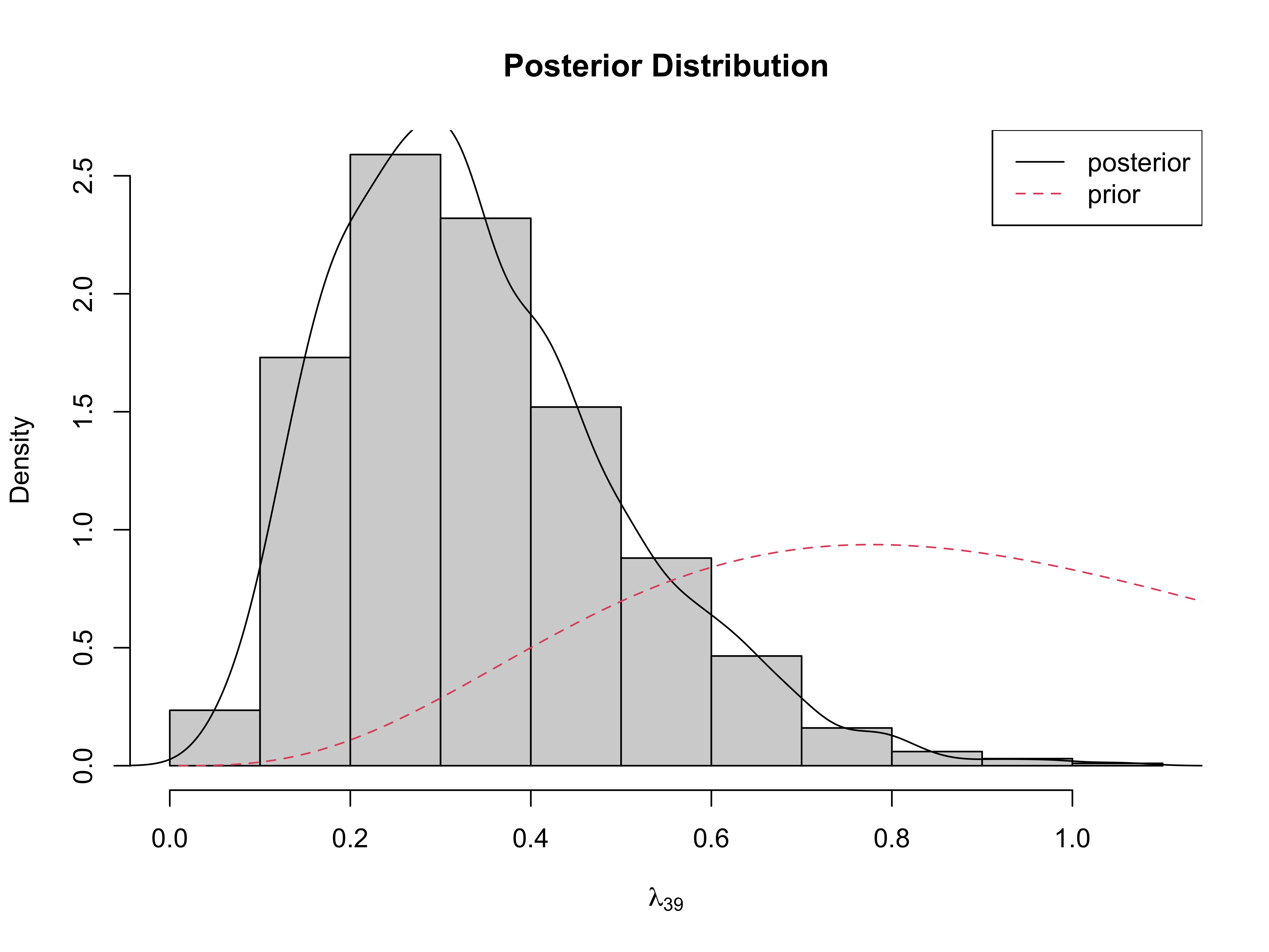
Posterior Distributions

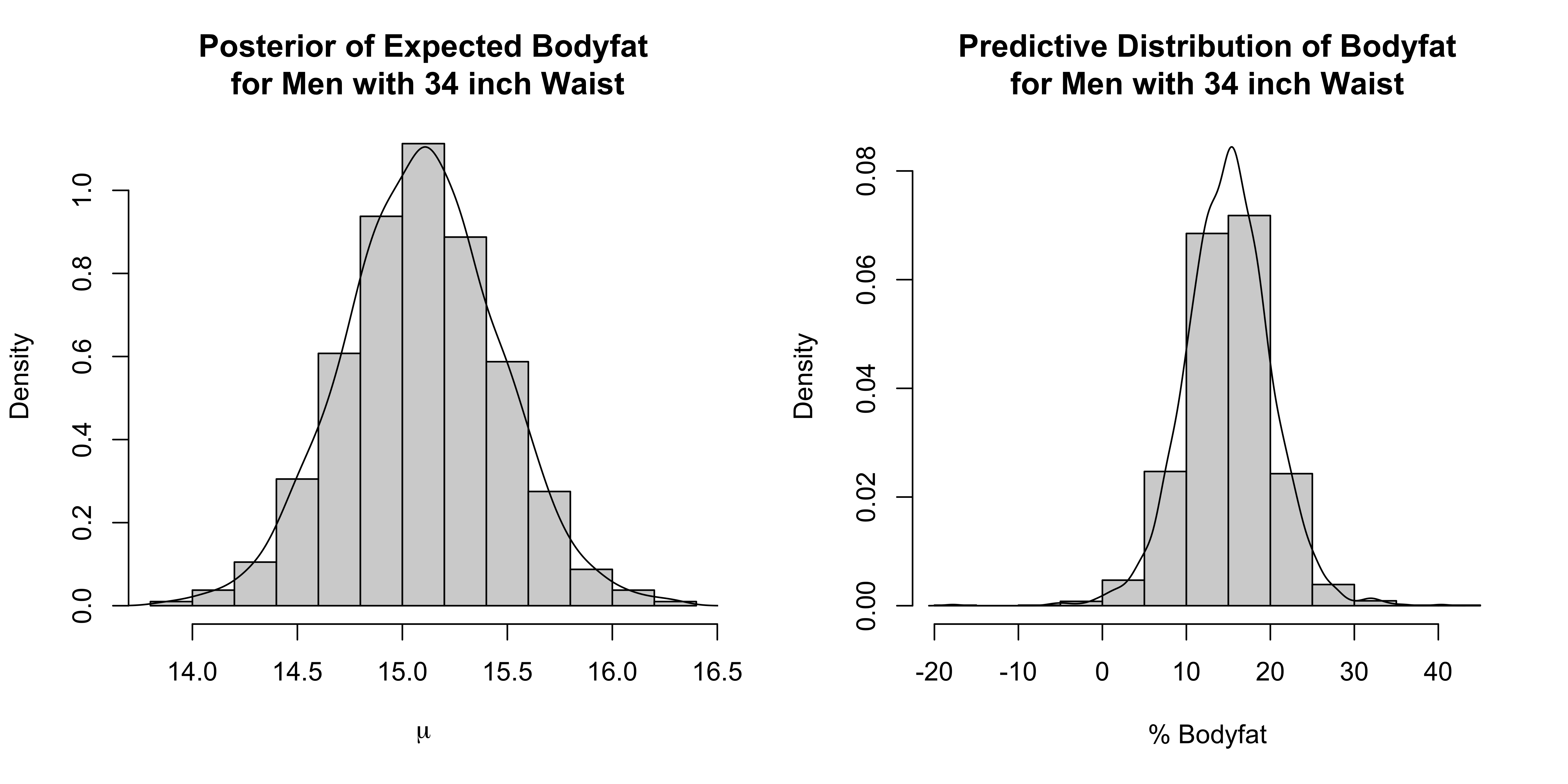
Posterior of \(\lambda_{39}\)

Comparison

95% Confidence/Credible Intervals for \(\beta\)

	2.5 %	97.5 %
lm all	0.5750739	0.6875349
robust bayes	0.5974085	0.7186084
lm w/out 39	0.6144288	0.7294781

• Results intermediate without having to remove any observations!

• Case 39 down weighted by \(\lambda_{39}\) in posterior for \(\beta\)

• Under prior \(E[\lambda_{i}] = 1\)

• large residuals lead to smaller \(\lambda\) \[\lambda_j \mid \text{rest}, Y \sim G \left(\frac{\nu + 1}{2}, \frac{\phi(y_j - \alpha - \beta x_j)^2 + \nu}{2} \right)\]

Prior Distributions on Parameters

• As a general recommendation, the prior distribution should have ``heavier’’ tails than the likelihood

• with \(t_9\) errors use a \(t_\alpha\) with \(\alpha < 9\)

• also represent via scale mixture of normals

• Horseshoe, Double Pareto, Cauchy all have heavier tails

Summary

• Classical diagnostics useful for EDA (checking data, potential outliers/influential points) or posterior predictive checks

• BMA/BVS and Bayesian robust regression avoid interactive decision making about outliers

• Robust Regression (Bayes) can still identify outliers through distribution on weights

• continuous versus mixture distribution on scale parameters

• Other mixtures (sub populations?) on scales and \(\boldsymbol{\beta}\)?

• Be careful about what predictors or transformations are used in the model as some outliers may be a result of model misspecification!